Module StatFilter

Table of Contents

• Aim of module
• General description
• Parameter description
• Examples
  • Example 1:
  • Example 2:
  • Example 3:
  • Example 4:
  • Example 5:

See Also

opals::IStatFilter

Aim of module

Performs statistical filtering of raster datasets with a sliding kernel of arbitrary shape and size.

General description

The Module StatFilter takes an input raster file (parameter inFile) and for each pixel calculates a statistical feature (parameter feature) by considering the neighbouring pixels in a user-defined kernel environment (parameter kernelShape, parameter kernelSize). The resulting output is again a raster (parameter outFile) in GDAL supported data format (parameter oFormat). The same statistical features as for Module Cell are provided, enabling low pass filtering (smoothing), boundary value extraction (min/max), roughness estimation, etc. The following features are provided:

• min: lowest pixel within kernel area
• max: highest pixel within kernel area
• range: highest minus lowest attribute value
• nmin: n-th lowest pixel
• nmax: n-th highest pixel
• mean: mean (average) of all pixels
• median: median of all pixels
• sum: sum of all pixels
• rms: root mean square of all pixels
• variance: (sample) variance of all pixels
• stdDev: standard deviation of all pixels
• stdDevMAD: robust standard deviation estimator computed from the median of absolute deviations from the median of all pixels
• pcount: nr of valid (i.e. non-nodata) pixels
• pdens: ratio of nr of valid (i.e. non-nodata) pixels to the nr of kernel pixels
• quantile: p-quantile (p=0..1) of all kernel pixels
• entropy: (shannon) entropy, measure of information content
• minority: class with the lowest frequency (based on a histogram of all pixels within kernel area. The bin width can be specified after a ':'. Default value is 1). This is especially useful for integer-typed rasters where the pixel values represent e.g. class identifiers.
• majority: class with the highest frequency (as above).

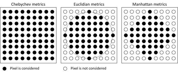
Depending on the application different neighbourhoods may be required. The following kernel shapes are supported:

• square: Chebyshev metrics
• circle: Euclidian metrics
• diamond: Manhattan metrics

Please note, that the kernel size is to be defined as a radius (in pixels) rather than as number of columns and lines. For a kernel radius of 4 (i.e. 9x9 kernel) the resulting kernels are shown in Figure 1.

Figure 1: Square, circle and diamond kernels

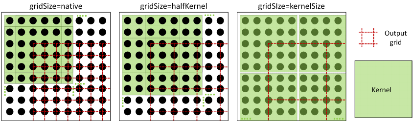
By default, the input and output rasters have identical structure, i.e. for each input pixel a corresponding output pixel (containing the statistically filtered value) is calculated and stored. However, it is also possible to manipulate the output grid resolution (gridSize. The follwoing otions are provided:

• gridSize=native: The output grid width corresponds to the input grid wdith
• gridSize=halfKernel: The output grid width equals the kernel radius size (i.e. half kernel size)
• gridSize=kernelSize: The output grid width equals the entire kernel size

Figure 2 illustrates the above mentioned resampling options:

Figure 2: Left: no resampling), Middle: output grid width = kernel radius, Right: output grid width = kernel size

Furthermore, the output grid extents may be changed by specifying a user defined limit (limit). Please note, that uneven limits are automatically rounded to the next grid post position. Optionally, a no-data value representing data voids in the output raster can be specified (parameter noData).

Parameter description

-inFileinput raster file

Type: opals::Path
Remarks: mandatory
Import raster image in GDAL supported format,

-outFileoutput raster file

Type: opals::Path
Remarks: estimable
Path of filtered raster image file in GDAL supported format.
Estimation rule: The current directory and the name (body) of the input file are used as file name basis. Additionally, the postfix and the extension are constructed accoding to the specified and oFormat (e.g. '_min.tif').

-oFormatraster file format [GTiff,AAIGrid,SCOP,...]

Type: opals::String
Remarks: estimable
Use GDAL driver names like GTiff, AAIGrid, USGSDEM, SCOP... .
Estimation rule: The output format is estimated based on the extension of the output file (*.tif->GTiff, *.dem->USGSDEM, *.dtm->SCOP...).

-featurestatistical feature

Type: opals::StatFeature
Remarks: mandatory
A statistical feature of the set [min,max,diff,nmin:n,nmax:n,mean,median,sum,variance,rms,pdens,pcount,quantile:p,minority,majority,entropy] is derived. For features nmin:n and nmax:n, n (>0) and for feature quantile p ([0,1]) must be specified

-kernelShapekernel shape

Type: opals::KernelShape
Remarks: default=square

Possible values:  
  square .... square kernel (Chebyshev metrics))
  circle .... circular kernel (Euclidean metrics)
  diamond ... diamond kernel (Manhattan metrics)

To select a predefined shape of the (binary) kernel matrix.

-kernelSizekernel size (radius of kernel in pixels)

Type: int
Remarks: default=1
Kernel radius

-limit2D clipping window

Type: opals::GridLimit
Remarks: optional
If no user defined limits are specified or -limit is even skipped, the entire xy-extents of the input raster model are used.

-noDatanodata value

Type: float
Remarks: default=9999
Value representing an undefined value in the output raster model

-gridSizeoutput grid size/resolution

Type: opals::GridResolution
Remarks: default=native

Possible values:  
  native ....... output grid size equals native input grid size
  halfKernel ... output grid size equals half kernel size
  kernelSize ... output grid size equals entire kernel size

By default, the output grid is calculated using the native input grid resolution. However, as the input pixels are used reduntantly for neigbouring output pixels in this case, a reduced resolution (half or entire kernel size) can be chosen. Especially for an output resolution corresponding to the kernelSize each input pixel is contributing to the resulting output grid one-time-only.

Examples

The following examples rely on the surface grids first.tif and last.tif derived from all first/last echoes of the dataset fullwave.fwf as described in Example 3: (Example 3) of module Module Grid.

opalsImport -inf fullwave.fwf -iFormat FWF
opalsGrid -inFile fullwave.odm -outFile first.tif -filter Echo[First] -gridSize 0.5 -interpol movingPlanes
opalsGrid -inFile fullwave.odm -outFile last.tif  -filter Echo[Last]  -gridSize 0.5 -interpol movingPlanes

Example 1:

By averaging all pixels within the kernel area, low pass filtering (i.e. smoothing) of raster datasets can be performed. The smoothing level can be controlled by the kernel size.

opalsStatFilter -inFile first.tif -outFile smooth_weak.tif   -feature mean -kernelSize 1
opalsStatFilter -inFile first.tif -outFile smooth_medium.tif -feature mean -kernelSize 2
opalsStatFilter -inFile first.tif -outFile smooth_strong.tif -feature mean -kernelSize 3

This corresponds to a kernel size of 3x3, 5x5, and 7x7 resulting in gradually higher smoothing rates. Please note, that since the kernel shape is not explicitly defined, the square kernel is used by default.

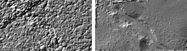
Example 2:

opalsStatFilter -inFile first.tif -outFile dsm.tif  -feature max -kernelSize 3 -kernelShape circle
opalsStatFilter -inFile last.tif  -outFile dtm.tif  -feature min -kernelSize 5 -kernelShape circle 

In this example, the min/max features are used to derive a DSM and DTM. In this example, the highest values of first-echo-surface model and the lowest values of the last-echo-surface model are filtered using circular kernel environment (euclidian metrics), resulting in a simple DSM and (very noisy!!) DTM. A hill shading of the two models is shown in Figure 3.

Figure 3: Left: DSM, max-filter based on first echoes, Right: DTM, min-filter based on last echoes

Example 3:

opalsStatFilter -inFile first.tif -outFile dsmGrid.tif  -feature max -kernelSize 2 -kernelShape circle -gridSize halfKernel

In this example the parameter gridSize=kernelSize is used to resample the output grid. The resulting grid has a grid width of 1.0 x 1.0m² (i.e. native grid width of 0.5m x kernel radius of 2 pixels).

Example 4:

opalsStatFilter -inFile first.tif -outFile dsm_kerneSize.tif  -feature max -kernelSize 2 -kernelShape circle -gridSize kernelSize

In this example the parameter gridSize is set to the entire size of the kernel resulting in a grid with a cell size of 2.5 x 2.5m².

Figure 4: Left: DSM, max-filter based on first echoes, Right: Resampled DSM (grid size = half kernel size = 1m)

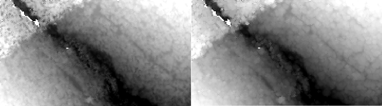
Example 5:

opalsStatFilter -inFile first.tif -outFile dsm_limit.tif  -feature max -kernelSize 1 -kernelShape circle -gridSize native -limit "(24790 311170 24980 311286)"

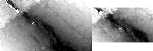
This example shows how to use the limit parameter. The result is sillustrated in Figure 4 below.

Figure 5: Left: DSM without limit, Right: DSM restricted to a user defined area-of-interest

Author

gm

Date

23.06.2016