Technische Universität Wien
Orientation and Processing of Airborne Laser Scanning data
Department of Geodesy and Geoinformation - Research Groups Photogrammetry and Remote Sensing
This page describes how different techincal aspects are handled and defined within OPALS.
In OPALS the terms grid and raster are used synonymously. However, you may observe a different interpretation when using center or corner in conjuction with the -limit parameter which is described in details below.
A grid or raster can be used to represent e.g. a digital terrain model (DTM) or digital surface model (DSM) inside a certain region of interest (ROI). Fig.1(a) shows a rectangular ROI with limits (Xmin, Ymin,Xmax,Ymax); see also FAQ on limit specification. Grid and raster are used synonymously. It is a set of regularly distributed 2D points with heights. The points are evenly spaced in X and Y by e.g. a distance s. Thus the grid for the ROI in Fig.1(a) would be given by Fig.1(b).
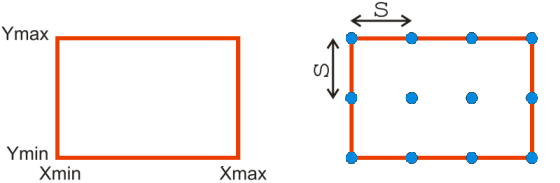
Note that the border points of the grid lie on the ROI limits. This is naturally required, as for different products (e.g. contour lines) heights need to be computed also at locations in between the grid points using interpolation. Outside the border points (and thus the ROI limits) no interpolation is possible - only extrapolation, which should be avoided in any case, because of unpredictable and unreliable results.
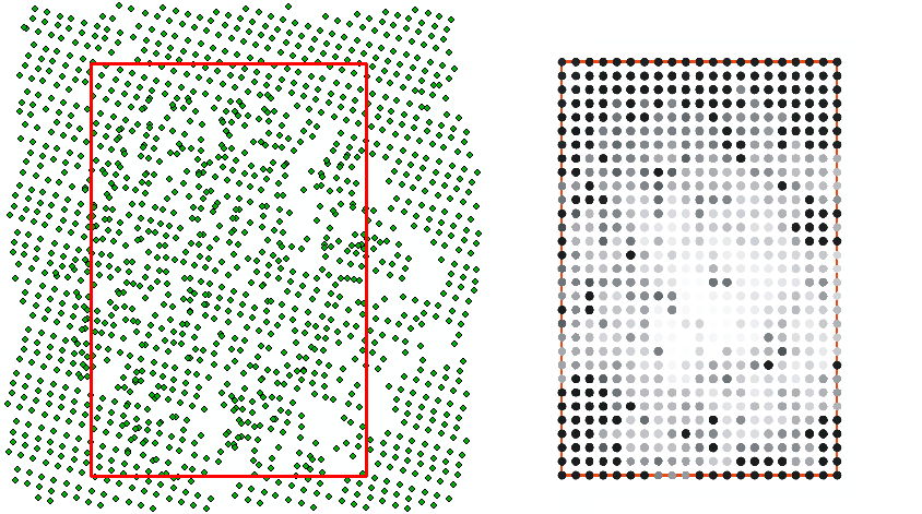
The direct visualization of the height values of the DTM can be achieved using a color coding and would thus be a set of colored points; see Fig.2(a). However, to enhance the perception the colored points are usually replaced by colored pixels; see Fig.2(b). This color coded visualization as a raster image is a direct product of the DTM, because the stored heights are used as they are.
Note that, the centers of the border pixels are lying on the limits. Therefore, the area covered by the pixels exceeds the limits of the ROI by half a column in east and west, and also by half a row in north and south. If only a single ROI is considered, then this exceeding is of no concern, usually. However, the exceeding may be unwanted in case of tiles. Tiles are rectangular ROIs, which are used to partition a larger area like a whole country into smaller parts for easier handling. Neighboring tiles do not overlap but lie gapless side by side. Therefore, also the color coded tiles of the DTM may be wanted to lie gapless side by side. For this purpose the raster image of the color coding should be created inscribed, so that the edges (and corners) of the border pixels lie on the ROI limits.
All OPALS modules provide the -limit parameter to control the location of the border pixels with respect to the input ROI limits. The input ROI limits are defined by the border points of the input file(s). As default (or by using the -limit parameter with value center) the output is generated so that the centers of the output border pixels lie on the input ROI limit;see Fig.3(a). Use the -limit parameter with value corner to place the edges (and corners) of the border output pixels on the input ROI limit (as maybe wanted in the case of tiles);see Fig.3(b). Note that in this latter case an interpolation is required and thus not the originally stored height values are used for the color coding.
opalsZColor using -limit center (=default) (same as Fig.2(b));opalsZColor using -limit cornerShading is another type of visualization. There the surface normal is needed in each point, which requires an interpolation in any case.
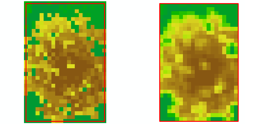
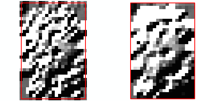
In the following figures the effect of the -limit parameter with values center (=default) and corner are demonstrated in another example using color codings (note the smoothing effects for the corner outputs in Fig.5(b) due to interpolation) and shadings. Fig.4(a) shows a section of ALS points around a tree together with the limits of a ROI. Fig.4(b) shows the grid of that ROI obtained from the ALS points using Module Grid with the nearest neighbor interpolation. Fig.5(a) and (b) show the output of opalsZColor using using -limit center (=default) and using -limit corner respectively. Fig.6(a) and (b) show the respective output of opalsShade.
Module Grid using nearest neighbor interpolation (grid points are grey colored)
Observe: If the corner output created in the above example (i.e. Fig.5(b) or Fig.6(b)) would be used as input again for an OPALS module the input limit would be smaller by half a pixel (on all four edges) compared to the original grid used for this example.
Extrapolation refers to estimating values beyond the range of observed data. As such, it involves greater uncertainty and carries a higher risk of producing unreliable or meaningless results.
OPALS provides various interpolation methods to convert point clouds into raster models. Some of these methods, such as Delaunay triangulation, are inherently resistant to extrapolation. Others, however, are more or less susceptible to extrapolation artifacts. For moving least-squares interpolation methods, the degree of extrapolation largely depends on the spatial arrangement of the input data. If the interpolation point is well surrounded by nearby data points, little to no extrapolation is expected. In contrast, extrapolation typically occurs when data points are located only on one side of the interpolation point. This situation commonly arises near data gaps or at the boundaries of datasets (e.g. at edge of flight strips), where the lack of surrounding observations increases the likelihood of extrapolation effects.
One approach to mitigate this issue is to ensure a homogeneous distribution of data points around the interpolation point, for example by using quadrant data selection as described in section Data selection strategies. A drawback of this method is its significantly higher computational cost compared to standard nearest neighbor selection. To address this, OPALS provides an additional strategy to largely avoid extrapolation without relying on computationally expensive data selection algorithms. In this approach, the interpolated value is checked against the value range of the input data.
\(\Delta_{v}=(v_{max} - v_{min}) \cdot tol_{rel} + tol_{abs}\)
where \(tol_{rel}\) refers to the global parameter and tolerance_rel (default value: 0.05) and \(tol_{abs}\) to tolerance_abs (default value: 0.0001). If the interpolated value lies within the acceptance interval
\([v_{min}-\Delta_{v};v_{max}+\Delta_{v}]\)
it is classified as non-extrapolated. If it is outside the given interval its classified as extrapolated and therefore rejected (if the corresponding module parameter extrapolationCheck is activated).
Note that an appropriate value for \(tol_{abs}\) is required to account for minor numerical deviations, even in the case of perfectly planar input data. Although all input values may be identical, floating-point conversions (with varying precision) as well as numerical instabilities in matrix inversion can introduce small deviations from these values.
If the extrapolation check is activated and values are classified as extrapolated, the module (e.g., Module DTM) will output a message similar to the following at the end of its processing:
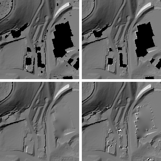
The effectiveness of the extrapolation check is clearly illustrated in Figure 7. First, a DTM was computed using Module DTM, both with (top left image) and without (top right image) the extrapolation check enabled. The resulting shaded DTMs are shown in the top row of Figure 7. At first glance, enabling the extrapolation check may appear disadvantageous, as fewer grid points are computed. However, when applying Module FillGaps with identical settings to both models (bottom row), interpolation artifacts at the edges of building gaps become clearly visible in the model without extrapolation control (bottom right image).
This observation reflects the interpolation philosophy adopted by OPALS: interpolation should only be performed at positions where reliable values can be ensured, while remaining gaps should be handled in a separate post-processing step if necessary.
 1.8.17