Table of Contents
- See Also
- opals::IGridFeature
Aim of module
Derives feature models (slope, curvature, roughness, etc.) from grid models based on the local grid neighbourhood defined by a kernel.
General description
Apart from the terrain height, Digital Terrain Models allow the derivation of additional features based on the local grid neighbourhood. Important features are, for instance, the terrain slope and curvature. Although the most accurate results are obtained by deriving these features as a by-product of the surface interpolation using the original point cloud in Module Grid, there are a couple of advantages for deriving these features on raster basis:
- the neighbourhood queries are much faster on grid basis compared to the point cloud
- the data distribution in the grid is regular (optimal for feature derivation)
- sometimes, only the interpolated grid is available but not the original point cloud
- etc.
The grid features are derived by taking all grid pixels into account within a certain kernel environment defined by its size (kernelSize, i.e. the kernel radius) and its shape (kernelShape, i.e.: square, circle, diamond). The following figure illustrates some standard cases:
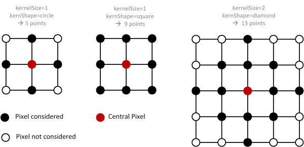
In general, the features are derived based on an appropriate underlying functional model. All slope related features, for instance, are calculated based on the best fitting plane defined by all valid grid points within the kernel. Curvature related features, in turn, are derived from a best fitting paraboloid. Multiple features can be calculated simultaneously simply be specifying a list of grid features (feature).
The following features are supported:
| Feature | Derived from | description |
|---|---|---|
| sigmaz | Plane | sigma z of grid post adjustment (i.e. std.dev. of the interpolated height) |
| sigma0 | Plane | sigma 0 of grid post adjustment (i.e. std.dev. of the unit weight observation) |
| slope | Plane | steepest slope [%] |
| slpDeg | Plane | steepest slope [deg] |
| slpRad | Plane | steepest slope [rad] |
| exposition | Plane | slope aspect [rad] (azimuth of steepest slope line, N=0, clockwise) |
| normalx | Plane | x-component of surface normal unit vector |
| normaly | Plane | y-component of surface normal unit vector |
| kmin | Paraboloid | minimum curvature [1/unit] |
| kmax | Paraboloid | maximum curvature |
| kmean | Paraboloid | mean curvature: kmean=(kmin+kmax)/2 |
| kgauss | Paraboloid | gaussian curvature: kgauss = kmin*kmax |
| kminDir | Paraboloid | direction (azimuth) of minimum curvature [rad] |
| kmaxDir | Paraboloid | direction (azimuth) of maximum curvature [rad] |
| absKmaxDir | Paraboloid | direction (azimuth) of maximum absolute curvature [rad] |
For each specified feature a separate grid file is calculated. The output grid file names (outFile) can either be specified explicitly, in which case a user-defined file name has to be specified for each feature. In case no or only file name is specified, unique file names are automatically created by adding the eature name as a postfix. The output grid files containing the feature rasters are created in GDAL supported format (oFormat). Please note that the feature grids are created in the same structure (resolution/extent) as the input DTM (inFile). Optional user defined limits can be specified to restrict the area of interest (limit). Please note that, irregular limits are automatically aligned to the grid structure of the input raster as re-sampling is strictly avoided.
Parameter description
Remarks: estimable
Path of filtered raster image file in GDAL supported format.
Estimation rule: The current directory and the name (body) of the input file are used as file name basis. Additionally, the postfix and the extension are constructed according to the specified grid feature and oFormat (e.g. '_slope.tif').
Remarks: estimable
Use GDAL driver names like GTiff, AAIGrid, USGSDEM, SCOP... .
Estimation rule: The output format is estimated based on the extension of the output file (*.tif->GTiff, *.dem->USGSDEM, *.dtm->SCOP...).
Remarks: mandatory
Possible values:
  sigma0 ....... sigma 0 of grid post adjustment (i.e. std.dev. of the unit weight observation)
  slope ........ steepest slope [%]
  slpDeg ....... steepest slope [deg]
  slpRad ....... steepest slope [rad]
  exposition ... slope aspect [rad] (azimuth of steepest slope line, N=0, clockwise)
  normalx ...... x-component of surface normal unit vector
  normaly ...... y-component of surface normal unit vector
  kmin ......... minimum curvature
  kmax ......... maximum curvature
  kmean ........ mean curvature: kmean=(kmin+kmax)/2
  kgauss ....... gaussian curvature: kgauss = kmin*kmax
  kminDir ...... Azimuth [rad] of minimum curvature
  kmaxDir ...... Azimuth [rad] of maximum curvature
  absKmaxDir ... Azimuth [rad] of maximum absolute curvature
  precision .... grid post precision (derived from sigmaz, pdens and slope)
The grid feature models are created in the same format and structure as the basic (input) surface model are derived. Please note that if more than one output file is specified, the number of output file names must match the number of specified features
Remarks: default=square
Possible values:
  square .... square kernel (Chebyshev metrics))
  circle .... circular kernel (Euclidean metrics)
  diamond ... diamond kernel (Manhattan metrics)
To select a predefined shape of the (binary) kernel matrix.
Remarks: default=1
To specify the kernel radius. A value of 1 corresponds to a 3x3, a value of 2 to a 5x5, [...] kernel.
Remarks: optional
If no user defined limits are specified or -limit is even skipped, the entire xy-extents of the input raster model are used.
Remarks: default=9999
Value representing an undefined value in the output raster model
Examples
The following examples rely on the grid model albis.tif located in the $OPALS_ROOT/demo/ directory.
Example 1: Slope rasters
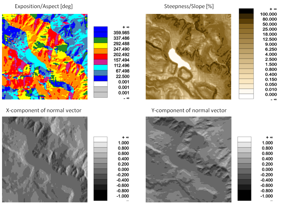
This first example demonstrates how to derive different slope feature grids (slope/steepness, exposition/aspect, x/y components of surface normal vector).
Since only the input file (albis.tif) and the feature list (slope, expos, normalx, normal) where specified, the default kernel settings (kernel radius: 1, kernel shape: square) were used. Consequently, for each grid point a best fitting plane was estimated using the grid point and its eight neighbours. The requested features are all calculated from this (tilted) plane. The names of the output grid files composed automatically based on the input file name and using the standard feature postfixes. (albis_expos.tif, etc).
The visualizations shown in Figure 2 are obtained with the following commands:
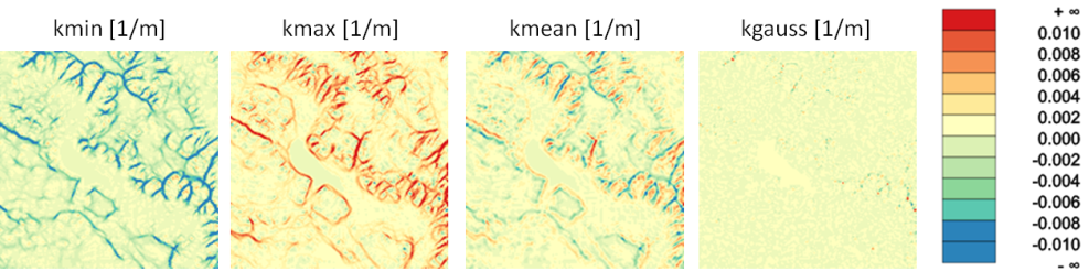
Example 2: Curvature rasters
In the second example different curvature rasters (minimum/maximum/mean/gaussian curvature) are derived. Hereby, a circular kernel shape and a kernel size (radius) of 2 pixels is used.
Figure 3 shows colour coded visualizations of the resulting curvature rasters which were derived using the following commands.
- Date
- 15.4.2014