Table of Contents
- See Also
- opals::IRobFilter
Aim of module
The aim of Module RobFilter is to classify the ALS point cloud (ODM) into terrain and off-terrain points based on robust surface interpolation
General description
Robust interpolation is a well established method for filtering ALS point cloud data (i.e. separation into terrain and off-terrain points). The basic concept of robust interpolation is:
- initial surface: First, an initial surface is interpolated using all equally weighted points (potentially considering a-priori weights)
- residuals/weights: Individual point weights are calculated based on the vertical deviations (i.e. residuals) of the ALS points w.r.t the current surface. In general, points above the surface get lower weights than points near or even under the surface. Thus, the surface is attracted to the lower (ground) points.
- enhancement of surface: A new surface is calculated considering the individual point weights.
- iteration: Steps 2 and 3 are repeated until the surface sufficiently approximates the terrain.
- classification: All points identified as inliers by the robust interpolation are classified as 'Ground' and the point classification set to ASPRS LASF Point Class 2). For all other points, the classification remains unchanged.
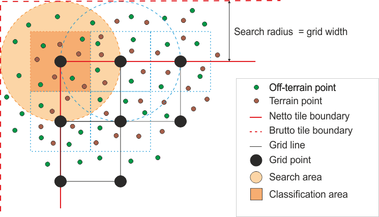
The overall processing sequence within Module RobFilter is grid oriented (c.f. Fig. 1). Based on the given search radius (parameter searchRadius) an internal grid is constructed (grid size = search radius). For each grid post location the local surface (parameter interpolation) is estimated considering all points within the search radius according to the scheme described above. If the accepted terrain points describe the estimated local terrain well enough, i.e. the standard deviation of the surface interpolation (sigma 0) is below a given threshold (parameter maxSigma), those points located within the raster cell around the respective grid location are re-classified.
Robust surface estimation tends to find the dominant surface model (parameter interpolation). In case that surface discontinuities (i.e. height jumps and/or slope changes) are dividing a local grid into more than one smooth region, the 2nd, 3rd, etc. most dominant surface is automatically searched. The decision to search for additional subareas is hereby made based on the analysis of the ground point distribution within a local processing unit.
The function for iteratively re-weighting the points is self adapting (considering the point density and distribution) but a user-defined function can also be specified explicitly (parameter weightFunc).
In general, the initial surface is calculated from all equally weighted points and, thus, describe an average surface but, however, a-priori weights can be considered in order to speed up the iteration process (parameter aprioiriWeight). The echo width parameter has proved to be a good pre-classifier, as a high echo width corresponds to a high vertical extension of the echo (bushes, trees, etc.). The generic filter syntax is used to specify the a-priori accuracy of a single point (echo), thus, all available point attributes can flexibly be combined for constructing a-priori weights.
Parameter description
Remarks: mandatory
The path to the opals datamanager whose point data are being classified
Remarks: default=plane
Possible values:
  plane ........ tilted plane
  paraboloid ... elliptic, circular or hyperpolic paraboloids
  adapting ..... adapting surface (prefers higher degree if necessary)
The interpolation methods are ordered by their polynomial degree. In case 'adapting' is chosen, a suitable interpolator is determined by the module, Higher degree interpolation is only used, if lower degree surfaces are too rigid.
Remarks: default=3
Only points within the given search radius are considered for the local robust interpolation.If the search area contains too few points for successful interpolation, the classification of the respective points remains unchanged.
Remarks: default=0.5
If the standard deviation of a unit observation of the robust interpolation (i.e. sigma_0 ) exceeds the specified value, the classification of the affected points remains unchanged.
Remarks: default=0.15
Either a constant accuracy representing all data points or a user-defined formula (using the generic filter syntax) may be applied. It is important thatthe a specified formula provide realistic accuracy values, otherwise therobust interpolation concept will not work properly.
Remarks: optional
If a filter string is specified, point classification is only carried out for the set points selected by the filter condition
Remarks: default=20
The laser signal is partly or totally reflected at semi-transparent objects like vegetation. Therefore, not all laser pulses reach the ground. The penetration rate is used in the course of the robust interpolation for apriori estimating a reasonable initial course of the local surfaces
Remarks: default=100
Robust interpolation is performed iteratively. In each iteration the individual point weights are adapted based on the residuals (i.e. vertical distance between point and intermediate surface. The process of surface interpolation and re-weighting is repeated until the surface changes are below a threshold or the maximum number of iterations is reached.
Examples
The following examples rely on the dataset fullwave2.fwf located in the $OPALS_ROOT/demo/ directory. As a precondition file containing full waveform data of a partially forested area needs to be imported into an ODM. Furthermore, a surface model is calculated used as comparison basis for the robust filtering examples below. Please use the following commands:
Example 1:
In the first example standard parameters are used to determine the ground points based on last echo point cloud.
The default parameters are used to perform the filtering (i.e., geometry model=plane, standard deviation of point heights=0.15m, search radius=processing grid size=3m). For visualization purposes the resulting set of ground points are additionally written to an XYZ ASCII output file (fwf_grdPts_defaultPars.xyz). Please note, that for all identified ground points the respective classification id corresponding to the LAS standard was set (i.e., classification=2). Please further note, that the classification ids are unchanged for all other points.
Example 2:
In this example the a-priori sigma of points is increased to an 0.25m. The consequence for the robust filtering is that more points are accepted as ground points. Before running the robust filtering again the classification is reset for all points.
Whereas the number of ground points was 51859 in the initial example, the count increased to 53547 using an accuracy of 25cm.
Example 3:
In this example the full waveform attribute EchoWidth is used to get rid of some remaining returns from shrubs and bushes. These returns are hard to distinguish using geometric criteria only, but often show an increased echo width as multiple targets within the laser footprint (i.e. ground ad shrub canopy) contribute to a single return with a broadened echo waveform. Using a filter, only echoes featuring a width less than 4.5ns are considered and further more echoes with a width of larger than 3ns are slightly down weighted by assigning a higher sigma a-priori.
It was only by this last example that also the low vegetation could be removed to a certain extent. This, in turn, caused a decrease of the ground point density, resulting in void pixels in the final DTM as can be seen in the following figure.

References
N. Pfeifer, G. Mandlburger: Filtering and DTM Generation; in: "Topographic Laser Ranging and Scanning: Principles and Processing", J. Shan, C. Toth (ed.); CRC Press, 2008, (invited), ISBN: 9781420051421, 307 - 333.