License

For the usage of the PCL a license of Opals is required.

Installation and Running

To use the PCL the installation of some python packages is required. The installation of those packages is done via the following command line:

pip install -r requirements.txt

For running the PCL please type:

python PointCloudLabeler.pyw

General Description

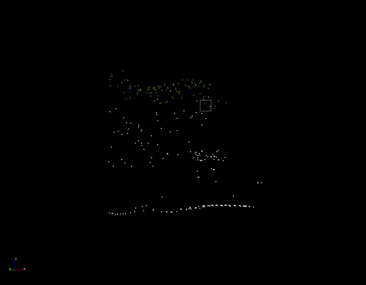
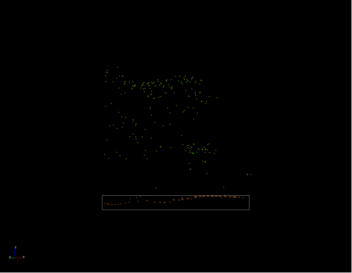
With the PCL it is possible to manually label 3D point clouds. To start the labeling process, the point cloud must be read in. Then an axis has to be defined. The labeling process is performed along this axis. It is possible to define several axes. Once an axis is defined, a polygon is created at the start of the axis. The polygon is normal to the axis. The extension of the polygon depends on the point density of the point cloud. The points inside the polygon are displayed as a vertical slice. This point can now be labeled. Once a section is labeled, it can be moved to the next section. To get a first prediction of the classes, it is possible to predict the classes of the unclassified points of the next section with a KNN tree (kNN - k Nearest Neighbors).

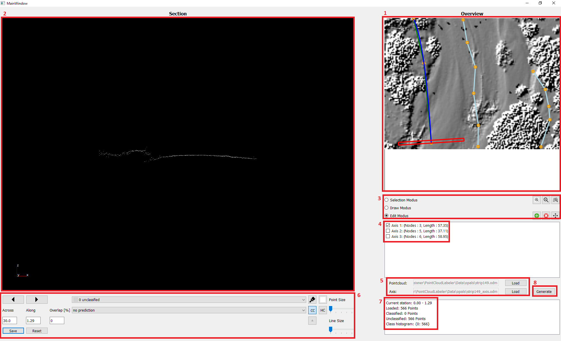
To get an overview of the whole area of the point cloud, a shading is displayed. This shading allows the definition of several axes. These axes can be used to navigate through the point cloud. The overview has a zoom and pan function. Use the mouse wheel to zoom in and out. To pan, press the left mouse button and drag over the shading (1). The PCL sequentially displays a portion of the full point cloud that can be classified (2). To change the active axis, select "Selection Mode". When this mode is activated, the active axis can be changed by clicking on the desired axis. To add a new axis, select "Draw Mode". An axis can then be simply drawn into the overview by clicking inside the shading. The vertices of an axis can be moved, deleted or a new vertex can be added to an axis. This is done by selecting the "Edit Mode". Use the three magnifying glass icons to zoom in and out (3). The different axes are listed with the corresponding information (the number of nodes and the lenght from the respective axis). The ceckbox of the currently active axis is checked. An axis can be deleted by right-clicking on it. The various axes, accompanied by the pertinent information, are enumerated. The deletion of an axis is initiated by right-clicking on the relevant item (4). In order to classify a point cloud, it is necessary to load the dataset. All data types that the Opals Datamanger can process are allowed. Once the data has been read in, it is possible to read in an existing axis datamanger (5). The panel can be used for classification, navigation and to display a greater or lesser number of points. The displayed section can be coloured either by class or by height. The different classes can be selected from a drop-down menu. When a section is classified, the classes of the following section can be predicted via a KNN tree (kNN - k Nearest Neighbors). The number of points displayed can be modified by adjusting the section geometry using the "Across" and "Along" numeric fields. The "Overlap" numeric field allows the user to define the degree of overlap between each section and its neighbours (6). To give a general overview of the displayed section of the total point cloud, some information is displayed. First, the current station of the section is displayed. The other information is about the points themselves (loaded points, classified points, unclassified points and a histogram of the classes) (7). It is possible to cover the whole area of interest with an axis (Axis Generation) (8).

Fig.1: PCL - PointCloudLabeler

Read in Data and define Axis

Fig.2: Read in the Data

The first line is the path to the laser scan data. The data can be in any format accepted by opalsImport. Once the point cloud has been imported and a shading is displayed we can now define the axes needed to navigate through the point cloud. This can be done in several ways:

QGIS: The axis can be defined in QGIS. In this case the axis needs to be saved as a shape file in the correct reference system. The path to the shape-file must then be entered in the second line.
Draw in shading: An axis can be drawn directly in shading. To do this, select the Draw mode. In the drawing mode we can easily draw the axis by clicking inside the shading. To confirm the axis, simply press the right mouse button. In the case of the first axis, a Save dialogue box opens. In this window the file name is required. The file is saved as an odm file. Once the file has been initialised, several axes can be added to the ODM. The ODM is automatically saved each time a new axis is confirmed.
Load ODM: An existing axis odm can be loaded directly. To do this, specify the path to the odm file in the second line.
Generate axis: If the whole area is to be covered, the generate option can be used. This will generate a large number of straight lines. First in a preview. In this preview the rotaion angle and the distance between the axes can be adjusted. The desired configurations must be confirmed. The generated axis is automatically saved as an odm file in the working directory.

Functions

kNN - k Nearest Neighbors

Once all points of the current section have been classified, you can select whether a prediction with kNN from the classes of the next section. For a prediction, an empty kdtree object is created with PointIndexLeaf, which represents a spatial leaf with a point index, is created. This kdTree object is filled with the points of the previous section. In the next step, the parameters are defined for how the prediction is to be carried out:

Parameters for kdtree object
Parameter	Value
nnCount	1
searchPoint	Coordinates of a point in the new section
searchMode	nearest
maxSearchDist	-1

With the point for which the class is to be predicted, the kdtree object is searched for its nearest neighbor. The maximum search radius is defined as -1. This means that the search continues until a nearest neighbor is found. If a neighbor is found, the class of the neighbor is assigned to the point. A prediction should only be made for those points that are not yet assigned to a class (equals to the value 0). To perform the prediction, select the different options (predict next, predict previous, always predict, no prediction) out of a dropdown menu.

Axis editing

For the editing of an axis the "Edit Modus" has to be turned on:

Fig.3: Active Edit Modus

The axis is stored as a linestring of coordinate tuples: [[x1,y1],[x2,y2],...]

Delete Vertices: To delete a vertex, click on or near the desired vertex. After the click, the mouse position is analysed to find the nearest vertex. When the nearest vertex is found, the pair of coordinates whose index is equal to the vertex number is removed from the linestring of the polyline.
Insert Vertices: To insert a new vertex, select the desired position in the shading. After the position has been selected, it is analysed which two vertices of the active axis are the nearest. If the two closest vertices are found, the coordinates of the new vertex are inserted into the line string of the polyline between the two vertices. Once the new vertex has been added, the splines for that axis are recalculated and the axis is redrawn in the overview graphics.
Move Vertices: To move a vertex, click and hold at or near the desired vertex. The click marks the vertex. To move the vertex to its new position, drag the mouse to any position on the shading and release the mouse button. The old coordinate tuple of the vertex is then replaced by the x,y coordinates of the mouse position where the mouse button was released.

Fig.4: Editing an Axis (from left to right): Original Axis, Delete of a Vetex, Insert of a Vertex, Move of a Vertex

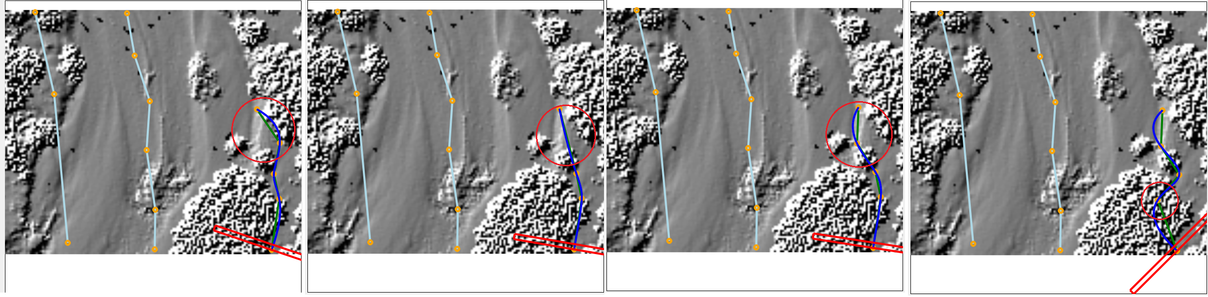
Note: It is only possible to edit the active axis!

Generate Axis

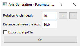
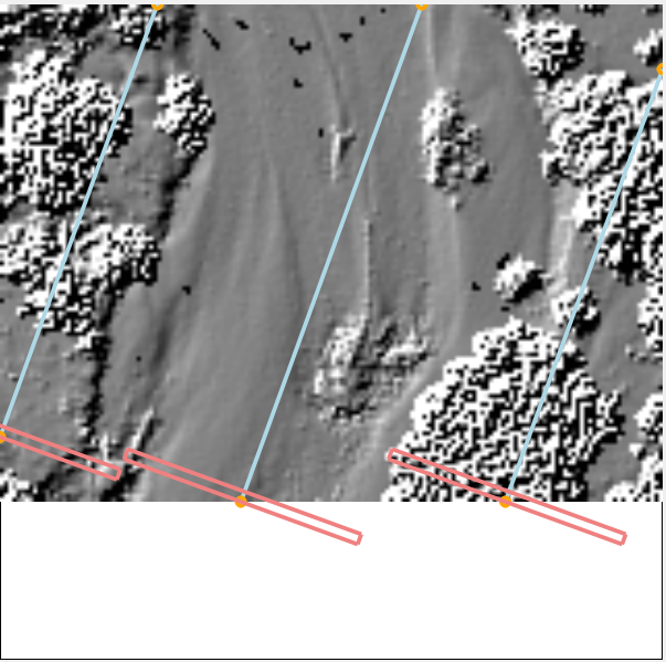
By generating axes, the entire area of interest can be covered. To do this, a polygon is created whose corner coordinates correspond to the coordinates of the corners of the area. In the next step, the centre point of this polygon will be evaluated. Once the centre point has been determined, the polygon is intersected by polylines. The distance between the polylines and the angle of rotation of the polylines can be adjusted. Each adjustment results in a preview for a first look at the area coverage. Note that the rotation angles are in degrees! Once the desired configuration has been selected it must be confirmed. It is also possible to export the polylines to a shape file.

Fig.5: Parameters for the arial coverage

Fig.6: Preview of the arial coverage

Examples

The data (strip149.laz) used in the following example is contained in the demo directory and read in.

Example 1: Classification

Dynamic Picker: The dynamic picker initially has a size of one pixel. If the mouse wheel is moved, the area of the mouse pointer is enlarged both horizontally and vertically in one step. A square is drawn around the pointer at the position where the mouse pointer is located. The size of the square depends on how often and in which direction the mouse wheel was moved. The square is displayed graphically in the widget. Once the appropriate size has been selected, it can be classified by left-clicking. All points within the square are assigned to the selected class. Another feature of this picker is that by holding down the left mouse button and left mouse button and moving the spanned square over points to classify them as with a brush. The area that is classified is the same as the spanned square.

Fig.7: Single Point Classification or Paint Multiple Points
Multipoint Picker: Marking several points is similar to the concept of the dynamic picker. The main difference is that the rectangle is drawn by holding down the left mouse button and moving the mouse. The current position of the mouse pointer on the widget is saved as the starting point. As long as the left mouse button is pressed and the mouse is moved, the rectangle changes size. If the left mouse button is released, the position of the mouse pointer is saved as the end position of the rectangle and all points within the rectangle are assigned to the selected classes. Like the dynamic picker, the rectangle is also displayed graphically.

Fig.8: Multiple Point Classification

Example 2: kNN Prediction

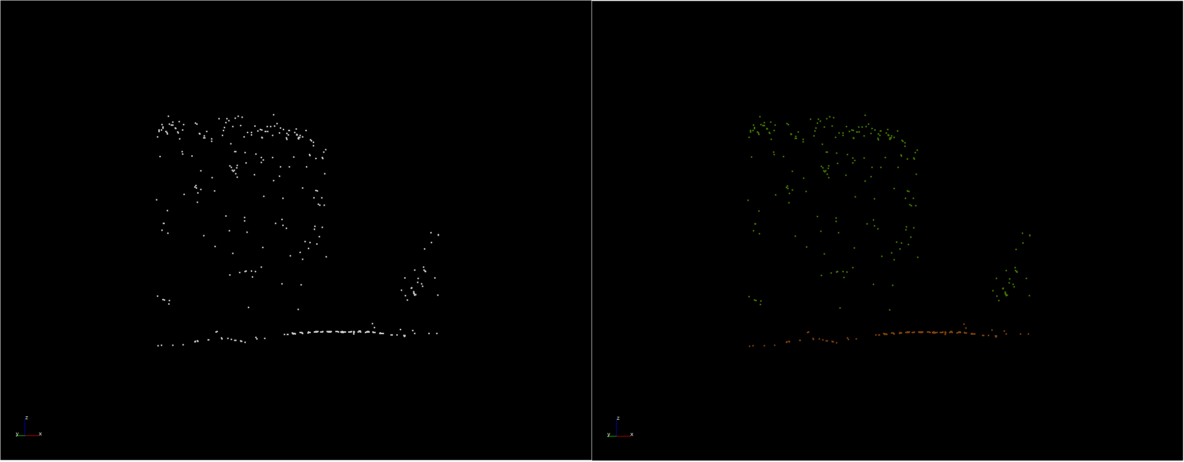
As mentioned before, it is possible to predict the classification for an unclassified section. This prediction is shown in Figure 9. On the left hand side no prediction has been selected. The predicted classification is shown on the right.

Fig.9: Next Section without Prediction (left), Next Section with Prediction (right)

Troubleshooting

The PCL is still in active development, therefore it can happend that the tool crashes sometimes. If you have trouble getting the PCL to run at all, here are couple of hints:

Use the most recent PCL version
Update OPALS to the latest nightly build
Check that your OPALS license is valid and in the cfg directory
Make sure that the axis are in the correct reference system

More information about the PCL can be find here: PCL Git Hub

Bugreports

Bug reports can be sent to the OPALS Team. Please include a short description of what you were trying to achieve, using what type of files, and the text from the error message. Copy-and-paste the messages printed to the console and include them in the bug report. Thank you!

Author: fmeixner

Date: 06.11.2024

Table of Contents