Technische Universität Wien
Orientation and Processing of Airborne Laser Scanning data
Department of Geodesy and Geoinformation - Research Groups Photogrammetry and Remote Sensing
In OPALS version 3 a new spatial neighborhood definition concept was introduced that unifies and extends the way for neighborhood descriptions in all OPALS modules. Whereas previously spatial neighborhoods were defined through various module parameters (neighbors, searchRadius, searchMode, ...) the new concept uses a descriptive syntax similar to filters linked to single parameter neighborhood. In spite of the unification not all options are available for all situations and modules. E.g. raster-based modules (e.g., Module Grid, Module Cell) are always limited to 2d queries whereas point-based modules (e.g., Module Normals, , Module PointStats, Module AddInfo) support both, 2d and 3d neighborhood definitions. The overall processing concept comprises the generic spatial neighborhood and optional processing and neighbor filters which are described at the end of this chapter. But let's start with the neighborhood definition.
The neighborhood definition always consists of a spatial query and some further optional properties. Currently, four different spatial queries are supported which can be categorized into two groups:
Although, it would be possible to support incremental queries directly on the point data, it can only be used in conjunction with sampling strategies for performance reasons. The generic spatial neighborhood concept uses a textual representation similar to the OPALS filter syntax. The representation is basically a concatenation of a query definition and optional expressions. Each expression consists of keyword (e.g. nn, window, incremental, etc.) with one value assigned (e.g. minPtCount=30) or additional options as key value pairs (key1=value1 key2=value2 â¦) within parentheses (e.g. knn(k=20 dim=3d)). The syntax supports abbreviation for keyword, keys and labelled values as long as they can be uniquely matched. As mentioned above, appropriate generic spatial neighborhood definitions depend on the module context and therefore, default values may vary from module to module.
To make neighborhood definition even more flexible, numeric values are not limited to fixed numbers. The spatial query also supports OPALS calculators which allows computing values based on attributes of the current processing point, e.g. circle(r=NormalizedZ*0.5+3) or based on values from raster files, which can be directly defined within the calculator syntax (more details to come). In case the calculator returns invalid, no spatial search is performed. Calculator formulae not containing white spaces or ':' characters are directly supported. In all other cases, formulae must be single or double quoted.
K nearest neighbor (kNN) queries are standard neighborhood definition for many applications. As in previous OPALS version kNN support quadrant and octant based kNN queries, meaning that neighbors are equally distributed across quadrants or octants (e.g. 8 neighbors in quadrant mode will secure 2 points in each quadrant). Quadrant or octant-based queries are beneficial when interpolating (avoids extrapolation), but on the other hand will result in significant lower query performance. For the sake of completeness, it is mentioned that the resulting neighbors are automatically sort based on the distance (2d or 3d depending on specified dimension) to the query point in ascending order.
knn(k=<>
  [dim=2d(default)|3d(default for opalsNormals)]
  [mode=omnidirectional(default)|quadrant|octant] )
For performance and memory reasons OPALS processes the data tile-wise and in parallel where each tile uses its own spatial point index (currently always a kd-tree). To avoid incorrect query results at the border of a tile, the local point indices are constructed with a certain overlap. Whereas the tile overlap can be calculated for fixed region queries, this is not possible for kNN queries. This is why previous OPALS versions requested a maximum search distance for kNN queries (By the way, a maximum search distance is beneficial to the performance of the kNN query itself as well). Nevertheless, in the new concept this is not explicitly requested any more, but can be implicitly provided by a combined kNN and fixed region query or by the maximum search distance parameter (see 1.2.4 for further details).
As it is for all numeric values, calculators are also support for defining value k. Floating-point values will be truncated to integer values and invalid results will ignore the current point for processing.
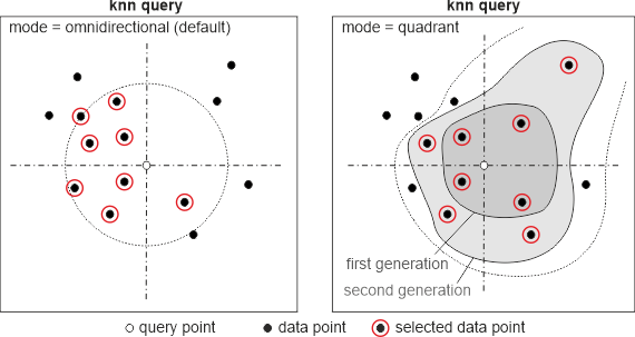
In quadrant-based mode the selected points are equally distributed among the four quadrants (NW, NE, SE, SW) around the (x,y) selection location (c.f. figure above), as long as, the number of neighbors is a multiple of four (4, 8, 12, ...). Hence, the first, second, third, etc. generation of quadrant neighbors are returned. If the number of neighbors has a remainder to 4, these "extra points" are also selected from different quadrants based on the distance criterion. In cases with empty (or inappropriate covered) quadrants this selection method only returns fully covered generation of quadrant neighbors, plus the appropriate number of extra points. E.g. if there are no points in two quadrants this method will always return 2 points (from the covered quadrants) even with higher number of neighbors than two. In octant mode the behavior is identical only switching from quadrants to octants.
knn(k=10 d=3d)
knn(k=8 d=2d mode=quadrant)
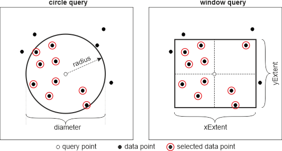
Fixed region queries are range queries as they have been supported in previous OPALS versions. Specified values refer to the full extent of the search region (i.e. the distance from the query position to the region boundary is half of specified value. compare Figure 2), except for circles, cylinders and spheres. There, the user can either specify the radius (half extent) or the diameter (full extent) of the region (see examples below). Although, it was possible to define a (asymmetric) range (rather than a single value) for the z component of a spatial search in previous versions of opals, the core-team has decided to discontinue this feature for two reasons: this feature had no practical relevance in the past and would complicate the syntax especially regarding the incremental search query. Secondly, supporting only z ranges implicitly focuses on coordinate systems with vertical axis and therefore, contradicts generic full 3d concepts.
window(xExtent=<> yExtent=<> | side=<>)
circle(radius=<>|diameter=<>)
box(xExtent=<> yExtent=<> zExtent=<> | side=<>)
sphere(radius=<>|diameter=<>)
cylinder(radius=<>|diameter=<> zExtent=<>)
sphere(r=30)  <=>  sphere(radius=30)  <=>  sphere(d=60)
box(s=2)
box(x=3 y=3 z=2.5)  <=>  box(xExtent=3 yExtent=3 zExtent=2.5)
cylinder(r=1 z=3)
The central idea of such queries is to provide neighbor definition similar to quadrant-based kNN but with a much higher performance. As mentioned above, those queries are only supported in conjunction with a sampling strategy where points are sorted into a cell matrix and the actual spatial query is then efficiently performed based on (full) cells. To support the kNN behavior (adapting the search distance based on the local point distribution) one has to specify a region query with ranges and increment (default=2 for extent/diameter and 1 for radius values. i.e. the query region is expanded by one cell size in each direction) and a minimum point count. Starting from the smallest region the extent of query is incrementally (by the defined value) increased until the maximum extent or minimum point count is reached. Please note that region values need to be specified in 'cell units'. E.g. circle(d=1) relates to one cell independent of sampling cell size. Currently only 2d sampling is supported meaning that regions are limited to 2d geometries (circle, window and square) as well. Ranges are specified with the slice operator as known from the OPALS calculator, python, or Matlab to define index ranges for sub-arrays or sub-matrices. First argument is the start value, second the included end value and the optional third value defines the increment. In this context one specifies extents rather than index ranges, which is why both values equally define the borders of the search region. Hence, start:end:inc can be interpreted as following C++ loop: for(double v=start; v<=end; v += inc) Note, the actual slice operator in the calculator syntax works differently: r[0:2] defines r[0], r[1] but not r[2].
Further details on how the spatial search exactly works in conjunction with sampling is presented in section sampling strategy.
incremental(<region query with range and optional increment>
  targetPtCount=<>)

incremental(circle(d=1:3) targetPtCount=30)
incremental(square(s=1:9:4) targetPtCount=50)
incremental(window(x=1:3 y=2:4) targetPtCount=15)
incremental(circle(d=1:3) targetPtCount=30)
It is possible to combine nearest neighbour and fixed region queries which results in a point set that is the intersection (=and) or union (=or) of both queries. Limiting kNN by region queries has usually a positive impact on the processing performance as well. Other combinations of neighbourhood definitions are not possible.
circle(d=3) and knn(k=20)
circle(d=3) or knn(k=20)
In general the or operator requires performing both queries on the full dataset and merging the results, whereas in case of the and operator only the first query is made within the full dataset and the second query is only applied on the first results. Whereas operator and allows implementing several static shortcuts (depending on region geometry and knn dimension), such shortcuts maybe also possible for the or operator but only in a dynamic way i.e. depending on the results of the first query.
A sampling strategy can serve different purposes but it was mainly implemented to improve spatial query performance. As described above, a sampling strategy is needed when utilizing incremental queries, but also fixed region queries are supported. Please note that region values are always interpreted in cell units when a sampling strategy was specified (otherwise values are interpreted with input data units).
A sampling can be also useful for homogenizing the point density or selecting specific points such as, highest point, point with smallest echo width, etc., before the actual processing step.
For point-based modules the sampling cell size is set by the cellsize parameter. For raster-based modules the subdivision parameter (only positive integer value are accepted) is the preferred way to do so. A subdivision value of 2 results in a cell size of half of the output raster cell size. Nevertheless, it is also possible to use the cellsize parameter for raster-based modules but possible values are limited. The output raster cell size must be a whole number multiple of the sampling cell size (i.e. 'raster cell size' modulo 'sampling cell size' == 0).
In general, there are three different ways of sampling the data:
sampling( cellsize=<>|subdivsion=<>
          [dim=2d (=default) | 3d]
          select=all | <statistic feature>(<optional parameters>)[<attribute>]
          [border=b  t  l  r  (default=bl)] )
sampling(cellsize=5 select=min[z])
sampling(cellsize=3.5 select=nmin(3)[z])
sampling(subdivsion=2 select=mean[z])
In the following the algorithm for spatial selection (in conjunction with a sampling strategy) is described. For point-based modules first the query point coordinates are transferred to the cell position. For grid-based modules the query location directly corresponds to the centre of a cell. Starting from those query cell centre position, the region query is applied. If a neighbouring cell centre is within the region, the cell is classified as neighbour and its content will be fully processed within the current query. If a cell centre is outside the region query, the cell will be ignored (even though it may partially overlap the query region). Hence, region queries in sampling mode are simply binary masks, which is why processing speed can be greatly improved.
The border parameter allows controlling the sorting behaviour of points that are lying on sampling cell borders. As default the bottom (b) and left (l) border of the cell are consider as cell part, resulting in a unique mapping of points to cell. However, this can lead to biased results in certain situation which is why different border handling strategies are supported. One can explicitly list which of the borders bottom (b), top (t), left (l) and right (r) should be assigned to the cell. Hence, it is possible to exclude (border=) or include (border=btlr) the all borders to a cell. Using those strategies, border points are either ignored or considered multiple times for processing.
For particular situations it useful or necessary that queried points are sorted in a certain order based on the distance to the query point or based on attribute values. Whereas kNN queries automatically return the points in ascending distance order (2d kNN based on 2d distance and kNN based on 3d distance) this might be relevant for fixed distance or incremental queries as well. The implementation automatically omits sorting if this is already done by the actual spatial search.
sort( (dist=2d | 3d)  | (attribute=<>)
      [order=asc(=default) | desc] )
knn(k=30 dim=2) sort(dist=3d)  ...performs a 2d kNN query but sort the points based on the 3d distance
circle(r=4) sort(d=3d o=desc)  ...performs a fixed distance query with radius 4 and sort points based on
                                  3d distance in descending order. Hence, n[0] is the farthest point
within the query regionFor certain processing strategies, it is necessary that at least a certain number of neighbours were found. This can be secured by the following option:
minPtCount=<>
This feature is e.g. useful to secure a certain robustness for the local normal estimation. Although only three neighbours are required to estimate a normal vector, the lack of redundancy prevents a quality estimation. E.g. using minPtCount=6 will most likely result in less normal vectors but for all vectors their sigma values can be computed.
The maximum search distance defines the leaf overlap when building the local kd-trees. This value is strictly optional and only comes into play when a maximum search distance cannot be derived from the spatial query itself (in case of only nn-queries or when using calculators in fixed regions). In case no maximum search radius can be derived and no value was provided it is defaulted with the half tilesize of the ODM.
maxSearchDistance=<>
In the following different examples are provided. Please note that definitions in one line that are separated by '<=>' are the same query but with different notation.
Basic queries:
knn(k=20)
knn(k=30) maxSearchDistance=50
window(x=10 y=10) <=>  window(s=10)
box(x=3 y=3 z=3)  <=>  box(s=3)
box(x=1 y=1 z=2)
Queries with sampling:
circle(d=5) sampling(cellsize=0.4 select=max[z])
incremental(circle(d=2:4) targetPtCount=20) sampling(subdivision=2
  select=max[z])
incremental(circle(d=2:4) target=20) sampling(cellsize=0.4 select=max[z])
incremental(window(1:3) target=30) sampling(cellsize=1 select=all)
Combined queries:
circle(d=3) and knn(k=20 dim=2) sort(3d)
cylinder(r=2 z=1) or knn(k=20) sort(2d)
knn(k=10 dim=3) and circle(r=5) sort(dist=2d)
Queries with calculators:
circle(d=NormalizedZ*0.5+3)
cylinder(r=3 zExtent=Amplitude*0.2)
knn(k=round(_myAttrib) dim=3d) sort(attr=z order=asc)
Filters are powerful tools to control processing within OPALS. OPALS version 3 introduces new contextual neighbor filters which are described in the following that allow for even more advanced processing strategies.
Please note that filters can be misused to introduce additional spatial relations between processing and neighboring points. However, spatial conditions should be solely defined by the neighborhood definition for performance and conceptional reasons. From a conceptional point of view, filters sub-select the data (i.e. make only data fulfilling certain criteria available) and therefore, they do not interfere the generic spatial neighborhood definition. In case no filter is provided no sub-selection will be performed.
Modules that perform spatial processing typically support two filter parameters:
When processing a dataset the modules first check if the current point should be processed. If the point passes the process filter then all neighboring point based on the given neighborhood definition are determined. Next, the neighboring points are checked against the neighbor filter. The transpired neighbors are then given to the actual calculation algorithm e.g. the interpolation routine in Module Grid or the normal estimator in Module Normals.
For modules that perform a point-to-raster conversion like opalsGrid, opalsCell, opalsDSM, etc. the filter.process parameter is typically of minor interest since the processing point is typically a 2d raster point than rather an 3d point of the data set. However, a region filter of building boundaries or water body polygons for limiting or excluding regions in the output raster might be still a viable application of this parameter. Nevertheless, the true power of this parameters arises for point-based modules, such as opalsNormals, opalsPointStats, opalsAddInfo, etc. There, the filter.process parameter allows sub-selecting which data points should be touched by the calculation. E.g. computing normals for last echoes only or deriving statistical neighborhood information for points of a specific class. Those stand-alone filter examples have been possible with previous versions of OPALS but the new contextual neighbor filters allow relating the current processing point with its neighbors.
A contextual filter allows sub-selecting neighboring points based on the current processing point. Let's start with some typical use cases before going into details:
PointSourceId) for computing e.g. a strip-wise point density Whenever a neighbor filter refers to the processing point - named base point in OPALS terminology - the filter is called contextual in contrast to stand-alone filters which does not link to the base point. The following filter example only neighbors from the same strip as the base point and with an Amplitude above 50 will be selected.
generic[b.PointSourceId == PointSourceId and Amplitude > 50]
Although the Amplitude condition is a stand-alone one the overall filter is still considered as contextual by OPALS. This has consequences on the internal processing algorithm and subsequently also on the performance of the computations. Within OPALS spatial neighbor queries are typically applied on local thread-dependent kD tress. Hence, stand-alone filters can be applied when filling the local kD trees which results in lower point numbers in the kD tree and neighbor filters can be omitted during spatial querying resulting in optimal performance. Contextual filters, on the other hand, cannot be applied in advance leading to larger kD trees and more importantly needs to be check for each point during spatial neighboring query. Therefore, the filter must be evaluated many more times (than stand-alone filters) especially for larger neighborhood definition. Hence, contextual filter may result in much lower performance.
MAYBE TO COME: pseudo code diagram
 1.8.17