Table of Contents
- See Also
- opals::IDTM
Aim of module
Calculates a high quality Digital Terrain Model in hybrid grid structure (i.e. regular grid + structure lines).
General description
Airborne Laser Scanning (ALS) provides a dense set of points located at arbitrary positions. The point densities are typically in the range of 1-20 points per square meter. ALS is also capable of penetrating vegetation through small gaps in the foliage and, thus, can provide the ground beneeth the canopy. One of the main applications of ALS is therefore the derivation of Digital Terrain Models (DTM). Interpolating the terrain surface is, however, the final step in a complex processing chain starting with waveform analysis, 3D point cloud derivation (Package opalsPreprocess), quality assessment (Package opalsQuality), geometric and radiometric calibration (Package opalsGeoref), derivation of 3D structure lines (Package opalsGeomorph), and filtering ground and off-terrain points (Package opalsClassify). In general, geo-statistical interpolation strategies have proven to deliver the best results. Kriging or linear prediction, respectively, are so-called BLUE (best linear unbiased estimators), but they are computationally expensive. Dense ALS point clouds therefore justify the usage of simpler interpolation techniques like moving least squares. Module DTM, in particular, uses linear or quadratic functional models (i.e. tilted planes or paraboloids). For each grid point the neigbouring laser points are used to locally fit such basic models and the grid height is calculated from the resulting geometry primitive. In addition to the point cloud, explicit line information e.g. from semi-automatic 3D structure line modeling (cf. Package opalsGeomorph) is considered within the DTM interpolation. Please note, that whereas the final goal of Module DTM is the construction of a hybrid DTM structure consisting of a regular elevation grid (i.e. height field) and vectors (interlinked structure lines), up to know the line information is specifically used for the grid point interpolation whereas the DTM is stored as a regular raster.
A single or multiple OPALS Datamanger (ODM) files containing, both, point and line data constitute the main input for Module DTM (inFile). The DTM raster (outFile) is stored in a GDAL (GeoData Abstraction Library) supported format. The grid spacing (gridSize) should be chosen to match the laser point density. As a rule of thumg, approximately 1-4 laser points should be used for the height estimation of a single grid point. Specification of the size of the internal processing and storage units (tileSize) is optional. Wheras larger tile sizes improve the computation performance they also require more RAM storage resources.
The neighbourhood defintion is crucial for local surface fitting. Module DTM uses a generation based point selection strategy illustrated in Figure 1.
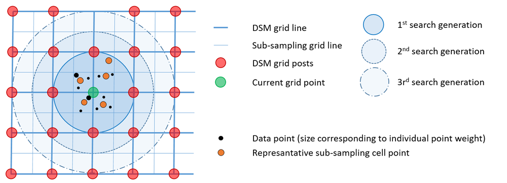
Data selection works as follows: The output grid structure is sub-sampled so that each output DTM grid cell is divided into four sub-sampling cells. The data points are then sorted into these sub-sampling cells. If more than one points falls within such a cell, a represantative point is calculated based on weighted center-of-gravity calculation. Therefore a user defined weight funtion can be specified (weightFunc). As a pratical example for this, the user might want to favor points with a higher (raw) amplitude or (calibrated) reflectance over points with low signal strength. In this case the respective point attributes (amplitude, reflectance, intensity, etc.) can directly used as weight function but, however, arbitrarily complex weight functions can be specified in gerneric filter syntax. Once all the points are sorted into the respective subsampling cell, the generation based point selection starts with a search radius equal to the DTM grid size. In the 1st> generation all sub-sampling grid cells with a maximum distance to the investigated grid post of 1 * DTM grid width are considered. If the number of neighbouring points is less then the requested knn-count (neighbours) the search radius is extended by one sub-sampling grid cell (i.e. half of the DTM grid spacing) and all points of the circular ring are added. The procedure is repeated until either the knn point count is greater than or equal (neighbours) or the maximum search radius (searchRadius) is reached. Please note that, although this is a raster based point selection approach, still the arbitrary positions of the representative cell points are maintained. In addition to the point data, all line data in the vicinity of the grid goint are considered within the interplation.
All remaining parameters are optional. As mentioned above, the primary aim of Module DTM is the derivation of a terrain model. Furthermore, additional feature models (feature) can be derived as by-products of the grid interpolation (i.e. without loss of performance). The following additional features are supported:
- sigmaz: std.dev. of interpolated grid height
- sigma0: std.dev. of the unit weight observation
- pcount: point count
- pdens: point density estimate
- excentricity: distance grid point - center of gravity of data points
- slope: steepest slope [%]
- slpDeg: steepest slope [deg]
- slpRad: steepest slope [rad]
- exposition: slope aspect [rad] = azimuth of steepest slope line, N=0, clockwise sense of rotation
- normalx: x-component of the surface normal unit vector
- normaly: y-component of the surface normal unit vector
- precision: heigth precision of grid post according to Kraus et al, 2006 (not yet supported)
By default, the entire ODM content is used as input. Specific point/line data selection is enabled by providing an appropriate filter string (filter). In addition, a user defined limit can be specified (limit). By default, the height raster and the additional feature rasters are written to separate files. To generate a single multi-band raster file set multiBand=1. Please note, that all raster files are created in GeoTiff file format and the individual rasters are kept together by a GDAL Virtual Raster master file. Future releases will extend this concept to implement a hybrid DTM structure (i.e. joint storage of both raster and vector contents).
Parameter description
Remarks: mandatory
The path(s) to the opals datamanager(s) whose point and line data are used to derive terrain model. In case multiple ODMs are specified, the data are queried from all (potentially overlapping) ODMs.
Remarks: estimable
Path of output DTM model file. Please note that the resulting DTM is stored as a hybrid raster. The regular grid of elevations and additional features are stored in GeoTiff format and the the structure information (spot heights, break lines, form lines, border lines) are stored in ESRI Shapefile format. If multiband output is enabled, a single raster output file containing the DTM grid and all features in separate bands (extension: '.tif') and a single vector file containing the stucture information (extension: '.shp') are created. If -multiband=false, a postfix is appended for each category (e.g. _dtm, _slope, _prec, _lines).
Estimation rule: The current directory and the name (body) of the input file are used as file name basis. Additionally, the postfixes ('_dtm', '_lines', ...) and extensions ('.tif' or '.shp') are appended.
Remarks: default=64
The internal processing is organized in rectangular tiles. The size of these computing units(number of grid lines per tile) can be specified allowing control of the memory consumption of the module. Recommended values are in the range of 64 (default) if the average point distance approximately matches the grid size. In case coarser or finer grids are to be derived, the tile size may need to be adapted. Finer grids allow for larger tile sizes (and vice versa).
Remarks: default=1
Size of the rectangular grid cell in x- and y-direction. If only one value is passed, quadratic cells are used.
Remarks: default=movingPlanes
Possible values:
  movingPlanes ... moving (tilted) plane interpolation
  kriging ........ kriging interpolation
Supported interpolation methods: movingPlanes|kriging.
Remarks: default=0
The neighbour search is performed raster based in 'generations'. First, a regular raster featuring half of the final cell size is derived (storing the CoG of all points in each cell). All (raster) points within a search radius of the final grid size are taken into account first. If there are less valid cells available than the required number of neighours, the search radius is extendended by half of the grid size. This procedure is repeated until either the required neighbour count is exceeded or the maximum search radius is reached. In case the minimum neighbour count is set to zero, all points within th maximum search radius are considered for interpolation of the grid height.
Remarks: estimable
Only points/lines within the given search radius are considered for the interpolation of a single grid post. If the search area contains too few points for successful interpolation, the respective grid point is omitted (void).Estimation rule: searchRadius = 3 * grid size.
Remarks: optional
An algebraic formula in generic filter syntax can be specified to calculate an individual weights for different classes of observations (bulk points, individual spot height points, soft structure line points (form lines), hard structure lines (break lines), and border lines. Please note, that additional point weights according to the distance of a data point w.r.t the grid post location are automatically calculated by the program to ensure a smooth terrain surface (i.e. inverse distance weighting).
Remarks: default=precision normalx normaly
Possible values:
  sigmaz ......... sigma z of grid post adjustment (i.e. std.dev. of the interpolated height)
  sigma0 ......... sigma 0 of grid post adjustment (i.e. std.dev. of the unit weight observation)
  pdens .......... point density estimate
  pcount ......... number of points used for interpolation of grid point
  excentricity ... distance between grid points - c.o.g. of data points
  slope .......... steepest slope [%]
  slpDeg ......... steepest slope [deg]
  slpRad ......... steepest slope [rad]
  exposition ..... slope aspect [rad] (azimuth of steepest slope line, N=0, clockwise)
  normalx ........ x-component of surface normal unit vector
  normaly ........ y-component of surface normal unit vector
  precision ...... grid post precision (derived from sigmaz, pdens and slope)
If one or more features are specified, additional grid models in the same format and structure as the basic terrain model are derived. By default, a multiband raster is created in this case. Please note, that if each feature is written to a separate file (i.e. multiband=false) and if more than one output file is specified, the number of output file names must match the number of specified features: nr. outFile = nr. feat. + 1
Remarks: optional
A filter string in EBNF syntax as described in section 'Filter syntax' can be passed to restrict the set of input points (e.g. to consider last echoes only).
Remarks: optional
If no user defined limits are specified or -limit is even skipped, the OPALS Data Manager (ODM) extents are used. Rounding is enabled by default in case the limits are derived from the ODM and can be enforced for user defined limits (keyword: round).
Remarks: default=0
When activated the resulting DTM grid and the selected feature rasters will be stored in a single multiband raster file instead of as multiple files. The single feature bands appear in the order of specification in the multiband raster file.
Examples
The data used in the following examples are located in the $OPALS_ROOT/demo/ directory. As pre-processing step, the 3D point cloud (flyover.laz) and the 3D break lines (flyover_breaklines.shp) are imported into a single ODM file using the following command:
To create a 25cm DTM grid based using 12 nearest neighbours in a maximum search distance of 1.25m and additional feature models (surface normal vector and grid height precision) use the follwoing command:
Visualizations of the resulting raster files (DTM shaded relief map, color coded sigmaZ, normalx and normaly map) are plotted in Figure 1:
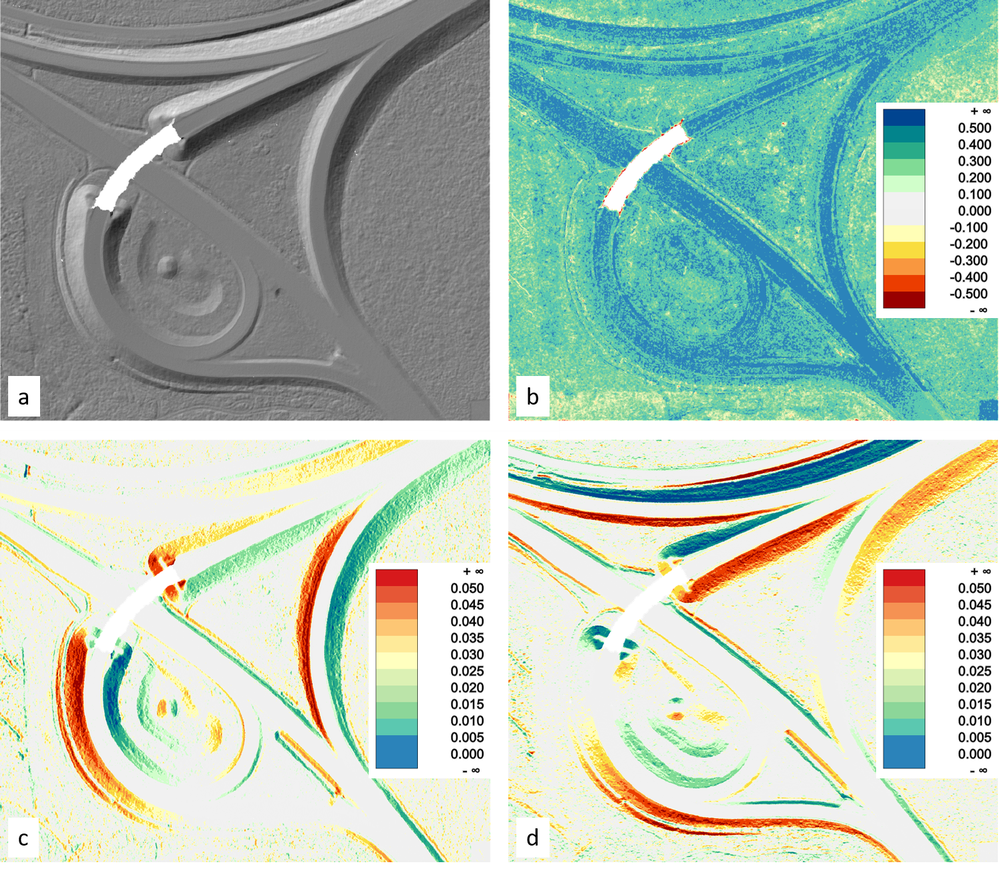
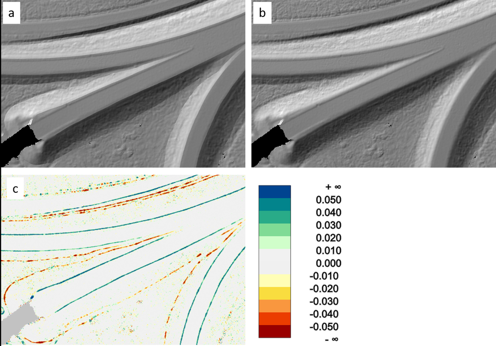
Figure 3 shows a detail of the shaded DTM relief compared to a variant without considering the breaklines in the surface interpolation (Module Grid):
References
- Date
- 2.12.2016