See Also: opals::IFullwave

Aim of module

Performs decomposition of the full waveform signal and provides 3D coordinates (scanner system) and additional attributes for each return.

General description

Laser scanners emit short laser pulses, which travel through the atmosphere, interact with the surface and the backscattered echo is detected at the scanners receiving unit. The range to the target can than be calculated from the time-of-travel of the laser signal. In discrete echo systems the echo detection is realized by hardware components whereas full-waveform scanners record the entire echo waveform, typically in 1 nanosecond intervals (c.f. Figure 1). This enables sophisticated signal analysis in the post processing.

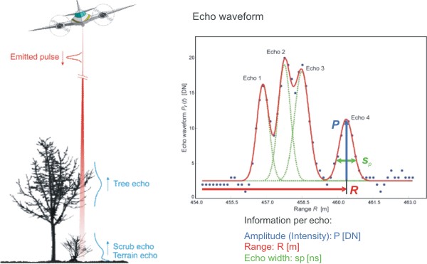
Figure 1: Full-waveform ALS, schematic diagram

The basic input for Module Fullwave is the raw full-waveform file (parameter inFile). Currently only Riegl Q-line instruments (e.g., LMS-Q 560/680i/780/1560) based on SDF (Sample Data File) are supported. The raw data are analyzed using the well-established method of gaussian decomposition. Gaussian decomposition provides the location (return time, range) as well as additional information about the signal strength (amplitude) and signal broadening (echo width) for each echo (c.f. Figure 1). For each extracted echo the following data fields are written to the output file (parameter outFile) either in an internal measure block oriented format (MB/SOCS) or in Riegl SDC (sample data coordinate) format (parameter oFormat):

X, Y, Z: echo coordinates in scanner system [m]
Time: GPS time of emitted laser pulse
Range: raw measured slant range value [m]
Rank angle: raw measured scan angle rank [deg]
Amplitude: amplitude estimated by gaussian decomposition [DN]
Width: echo width estimated by gaussian decomposition [0.1 ns]
echo number: echo index (i.e. i'th echo of a single laser pulse)
nr of echoes: total number of echoes of the current laser pulse

By default, the entire recorded waveform information is processed. However, the precessing can be limited to a certain range of pulses (timeRange). Additionally, the number of extracted echoes can be controlled via a detection threshold (detectThrLow).

Some scanners allow for multiple pulses in air (multiple-time around, MTA). This technique is supported by opalsFullwave

by applying a constant MTA zone offset (mtaZone>0) or
by automatically estimating the start zone and tracking the zone transitions (mtaZone=0); the start MTA zone is estimated in an energy-minimizing approach (c.f. Rieger and Ullrich, 2012; right of usage of patent AT511310B1 granted by Riegl LMS).

Parameter description

-inFilefullwave input filename

Type: opals::Path
Remarks: mandatory
From the specified fullwave input file echos are extracted. Supported formats: Riegl sdf and wfm files

-outFileoutput filename

Type: opals::Path
Remarks: estimable
Extracted echos are written in the scanner coordiante system to the output file.Estimation rule: The current path and the name (body) of the input file are used as file name basis

-oFormatouput file format [MB/SOCS|SDC]

Type: opals::String
Remarks: default=sdc
Estimation rule: The output format is estimated based on the extension of the output file (no extension -> MB/SOCS,*.sdc->SDC.

-fullWaveAlgfullwave algorithm

Type: opals::FullwaveAlgorithm
Remarks: default=gaussian

Possible values:  
  gaussian ........... Gaussian decomposition, standard
  asdf ............... ASDF only (no pulse width)
  enhancedGaussian ... Gaussian decompostion, ASDF echo detection

Note that echo width estimation is only supported for gaussian and enhancedGaussion but not for asdf(Averaged Square Difference Function).

-detectThrLowmin peak amplitude for detection of low channel echoes

Type: int
Remarks: default=200
Echoes in the low power channel are only detected if the peak amplitude [DN] is greater than the specified threshold.

-mtaZonedefines the MTA zone for multiple-time-around scanners

Type: int
Remarks: optional
For scanners supporting multiple-pulses-in-the air or multiple-time-around, respectively, (e.g LMS-Q-Q680) either a fixed MTA zone has to be defined to resolve distance ambiguities or the proper MTA zone has to be determined by analyzing (consecutive) waveforms:
mtaZone>0: processing of all laser echoes in the specified fixed MTA zone
mtaZone=0: automatic MTA zone detection based on analysis of consecutive waveforms

-timeRangetime limit in gps seconds for processing a subset only

Type: opals::Array<double,2>
Remarks: optional
If specified the data only wihtin the given gps time seconds are process. Use -1 as empty limit. Hence, it is possible to define an upper limit (e.g. -1 634.01) or a lower limit (e.g. 403.23 -1)

-filtermodify the input using a (tree of) filter(s)

Type: opals::String
Remarks: optional
A filter string in EBNF syntax as described in section 'Filter syntax' can be passed to restrict the output data set (e.g. output last echoes only)

Examples

All data used in the following examples are located in the $OPALS_ROOT/demo/ directory of the OPALS distribution.

Example 1

We start from the given demo file Dischmatal_fwf.sdf. First, Module Fullwave has to be applied to this file in order to generate the file Dischmatal_fwf.sdc, i.e. a point cloud in the Scanner's Own Coordinate System (SOCS):

opalsFullwave -infile Dischmatal_fwf.sdf -detectThrLow 10 -outfile Dischmatal_fwf.sdc -mtaZone 0

After this step, Module DirectGeoref has to be applied to transform the SOCS point cloud to a superior coordinate system, e.g. the corresponding UTM projection:

In this example, we have a Down-Front-Right scanner system (without tilting and time lag).

opalsDirectGeoref -inFile Dischmatal_fwf.sdc -outFile Dischmatal.fwf -trj Dischmatal_tra.txt -tFormat trajectory.xml -mounting "TIMELAG(0.0), SCANNERSYS(D-F-R), MOUNTROTATION=GLOBAL(ANGLES(0 0 0), AXISHIERARCHY(X-Y-Z), SENSEOFROT(CCW), UNITS(RAD)), MOUNTSHIFT=LOCAL(0 0 0)" -coord_ref_sys EPSG:32632

As result, we obtain the ASCII file Dischmatal.fwf containing the georeferenced point cloud.

Fig. 2: Point cloud extracted by OPALS FullWave, including MTA zone estimation and tracking

References

W. Wagner, A. Ulrich, V. Ducic, T. Melzer, N. Studnicka: Gaussian Decomposition and Calibration of a Novel Small-Footprint Full-Waveform Digitising Airborne Laser Scanner; ISPRS Journal of Photogrammetry and Remote Sensing, 60 (2006), 2; 100 - 112.

A. Roncat, G. Bergauer, N. Pfeifer: Retrieval of the Backscatter Cross-Section in Full-Waveform Lidar Data using B-Splines"; ISPRS Commission III Symposium PCV 2010 – Photogrammetric Computer Vision and Image Analysis, Paris (invited); in: "IAPRS Volume XXXVIII Part 3B", (2010), ISSN: 1682-1750; 137 - 142.

P. Rieger, A. Ullrich: A novel range ambiguity resolution technique applying pulse-position modulation in time-of-flight ranging applications. Proc. SPIE Vol. 8379 (2012). doi:10.1117/12.919140