Table of Contents
- See Also
- opals::IRadioCal
Aim of module
Performs radiometric calibration of ALS data and calculates physical quantities (backscatter cross section/coefficient, reflectance) for each return.
General description
Most classification techniques use the geometry of the 3D point cloud or parameters which can be gained from analyzing the geometry or a number of echoes per emitted laser shot (attributes EchoNumber and NrOfEchos when using the opalsInfo module). However, decomposing the echo waveform of full-waveform (FWF) ALS sensors can provide, in addition to the 3D position of each echo, its amplitude and echo width. These physical observables allow to study the radiometry of ALS data as they describe the power of the returning signal. They are influenced, though, by many different factors (e.g. range, angle of incidence, surface characteristics, atmosphere, etc.). Therefore, the comparability of these attributes between different datasets or even flight missions of different time periods is limited. By performing radiometric calibration, the amplitude and echo width are converted into absolute radiometric values, i.e. backscatter cross section, the backscattering coefficient (area-normalized), or diffuse reflectance measure (incidence angle corrected) all of which describing the characteristics of the observed surface. Classification, thus, becomes independent of sensor and mission parameters.
The process of radiometric calibration is based on the following LiDAR adapted formulation of the radar equation which describes the relation between the transmitted  and the received power
  of an ALS system:
![\[\mathbf{P_r}=\frac{\mathbf{P_t}\mathbf{D_r^2}}{4\mathbf{\pi}\mathbf{R^4}\mathbf{\beta_t^2}}\cdot\mathbf{\sigma}\cdot\mathbf{\eta_{sys}}\cdot\mathbf{\eta_{atm}}\]](form_175.png)
This formulation considers the following influencing factors: the receiver aperture diameter  , the range between the sensor and the target
  , the laser beam divergence
  , the backscatter cross section
  as well as losses occurring due to the atmosphere or in the laser scanner system itself, i.e. a system and atmospheric transmission factor
  and
and  respectively. The backscatter cross section, which is given by the formula below, combines all target parameters such as the laser foot area
  (i.e. the size of the area illuminated by the laser beam), the reflectivity
  , and the directionality of the scattering of the surface
  .
.
![\[ \mathbf{\sigma}=\frac{\mathbf{4\pi}}{\mathbf{\Omega}}\mathbf{\rho}\mathbf{A_i} \]](form_184.png)
All parameters which are unknown, but can be assumed to be invariant during one ALS campaign, can be summarized in one constant, the so-called calibration constant  . This is eventually mathematically described as:
![\[\mathbf{C_{cal}}=\frac{\mathbf{\beta_t^2}}{\mathbf{P_t}\mathbf{D_r^2}\eta_{sys}} \]](form_186.png)
Combining the first and third equation the formula for the backscatter cross section can be written as:
![\[\mathbf{\sigma}=\frac{\mathbf{C_{cal}}\mathbf{4\pi}\mathbf{R^4}\mathbf{\hat{P}_{iS_{p,i}}}}{\eta_{atm}} \]](form_187.png)
It is mentioned that in the above equation the actual received power is replaced by the term  . This is due to the fact that received power is proportional to the product of the amplitude
  and the echo width
  .
.
In order to achieve calibrated radiometric measures for the entire 3D point cloud, the Module RadioCal has to be applied twice. Based on the above equations describing the backscatter cross section, the ccalibration constant is derived for all single echoes within selected areas of known/measured reflectivity in a first run based on sensor data (range, amplitude, echo width, laser beam direction, cf. Module Import) and surface information (surface normal vector, cf. Module Normals). Those 2D calibration polygons can either be provided as shape or winput file(s) (see Definition of calibration regions for further details). The final calibration constant is then calculated by averaging the medians of each calibration region. If needed it is possible to output the calibration values extended points (within the calibration polygons) for further analysis. As shown in the example below, Module Histo can easily applied when storing the points as additional ODM.
In a second run of Module RadioCal the calculated calibration constant is applied to the entire point cloud and calibrated radiometric values are obtained for each echo. This process includes the estimation of the backscatter cross section, backscattering coefficients and incidence angle corrected values. The workflow for the absolute radiometric calibration of an ALS dataset can be summarized in the following figure:
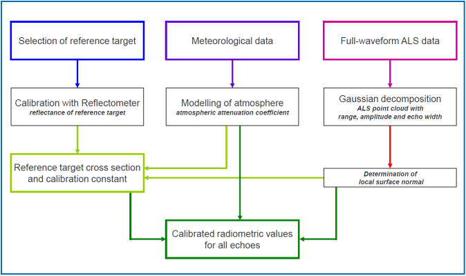
What follows is a short description of the output values (i.e. additional echo attributes stored in the OPALS Datamanager):
- _Sigma: is the backscatter cross section and combines the backscatter characteristics and the size of the target.
- _Gamma: is the backscattering coefficient and is the area-normalized version of the backscatter cross section and, thus, depends on the backscatter characteristics only.
- Reflectance: is an incidence angle corrected value. Thus, it requires the geometric modelling of the local surface normal in order to derive the angle of incidence for each echo. For echoes, where no local surface normal can be estimated or the plane fit does not satisfy certain quality criteria, the angle of incidence is set to zero. Furthermore, the assumption of diffuse reflectance behaviour is assumed for all surfaces. Thus, only for surfaces with Lambertian backscatter characteristics this value delivers the real reflectance of the surface. For non-Lambertian surfaces the value can be interpreted as diffuse reflectance measure at the specific measurement geometry.
Definition of calibration regions
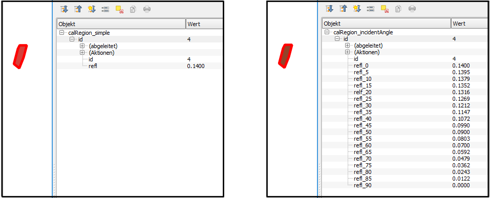
Calibration regions defined 2D polygon of known or measured reflectivity. If one reflectivity value per polygon is provided, Module RadioCal assume Lambertian backscatter characteristics and uses the Lambert's cosine law to compute the incidence angle depended values. If the backscatter characteristics of the calibration region doesn't follow an Lambertian surface, it is possible to describe its characteristics based on a table of incident angles and corresponding reflectivity values (linear interpolation is used in between the sampling points).
Using shape files
The widely-used shape file format can store arbitrary attribute values for each geometry object which perfectly suites the requirements for this use case. E.g. the open-source GIS QGIS can be used to create a corresponding polygon shape file, that contains (at least) an Id and a refl column (example: $OPALS_ROOT/demo/calRegion_simple.shp). For the non-Lambertian surface case multiple reflectance columns must be defined that follow the pattern refl_<angle> where angle has to be an integer value (example: $OPALS_ROOT/demo/calRegion_incidentAngle.shp)
Using winput files
If winput files are use to define calibration regions, reflectivity values needs to provided in a simple additional text file. Module RadioCal expects a specific naming of the text file based on the corresponding winput file: <filename>.wnp → <filename>_reflectivity.txt
Reflectivity values and geometry information are matched based on the given ids (2 digit winput code + 4 digit structure line number). As shown below each region is represented as column within the reflectivity text file (excerpt of $OPALS_ROOT/demo/calRegion_reflectivity.txt). For Lambertian surfaces only the zero incident angle row has to be provided.
Multiple calibration constants
Module RadioCal is capable of determining multiple calibration constants within a single run. This feature is useful if the data have been captured with multiple laser/detector units (e.g. Velodyne scanners) or the radiometric stability of a sensor such be investigated in case of multi epoch measurement campaign. As a prerequisite the input data have to contain a integral attribute which is internally used to split them into independent point sets. By setting the attribute name as splitByAttribute parameter, the module computes calibration constants for all uniquely occurring attribute values within the calibration regions. Hence, the output of the module is a calibration constant table rather than a single value. Full calibration details can be accessed from Python or C++ by querying the radioCal parameter. For the commandline is recommanded to make use of the parameter mapping concept of opals to pass the results of the first run of the module to actual calibration stage (see Example 2: Multiple calibration constant workflow for details)
Parameter description
Remarks: mandatory
Datamanager input file(s), which has to include the beam vector (see Module Import) and the normal vector for each point (see Module Normals)
Remarks: optional
If specified all points inside the calibration regions including new attributes are written to this file. The file format is estimated from the file extension, if not specified by the oFormat parameter.
Remarks: optional
Defines the file format for the optional region output file. Use 'odm' or 'RadioCalOutput.xml' for further analysis of the point data.
Remarks: optional
A filter string in EBNF syntax as described in section 'Filter syntax' can be passed to restrict the point used for calibration within the defined calibration regions
Remarks: optional
polygon calibration regions can be defined by winput file(s) with corresponding reflectivity files or by polygon shapefiles with corresponding reflectivity attribute columns.
Remarks: default=0
Atmospheric attenuation coefficient [0...1] calculated e.g. by IDL program calc_trans_lidar
Remarks: optional
beam divergence of the ALS system
Remarks: optional
Radiometric calibration constant derived by the first run of Module RadioCal
Remarks: optional
Compute different calibration constants based on values by the specified attribute. For each unique attribute value a separate calibration constant will be estimated (precondition: attribute type need to be integral)
Remarks: default=0.1
If a point has (no or) a NormalSigma0 value that is greater than given threshold, a vertical normal vector will be used. Use maxSigma <= 0 to deactivate the threshold check.
Examples
The data used in the following example can be found in the $OPALS_ROOT/demo/ directory. This example gives a guidance on how the opalsRadioCal module can be used for the absolute radiometric calibration of an ALS point cloud. A brief description of the required files (apart from the point clouds) is also included.
Example 1:
In order to perform the absolute radiometric calibration, the ALS point cloud data must be first imported into the ODM and the surface normals information per LiDAR echo must be computed (by performing local plane estimation). To achieve that, change to the demo directory and run:
The point clouds of two strips of the same flight are contained in the compressed LAS files, strip11.laz and strip21.laz. By specifying the the parameters -trjFile, Range, and BeamVector during data import the three components of the beam vector and the measurement range are automatically computed for each laser echo based on the flight trajectory and stored in ODM. In addition, the formats of the point cloud data as well as the trajectory file are specified by using the OPALS Format Definition XML files LAS_1.2_ew.xml and trajectory.xml respectively. In addition, the step of the normals calculation is required for the derivation of the reflectance described below. Here, the plane fitting considers the neighbourhood of 8 points in a maximum radius of 5 meters. In addition, by using the parameter -filter Echo [Last], only the last echo of each pulse is used (in case there are multiple targets).
What follows is the calculation of the calibration constant for the two strips seperately. Run the following command for both .odm files:
The module receives as input an .odm file that already contains all the necessary attributes. The output is an .odm file featuring all echos of the reference areas (calRegion.wnp) were reflectance measurements are available and contains the attribute _RadioCalConst, i.e. the calculated calibration constant, in addition to the existing echo attributes. In short, it is mentioned that the reflLambertian_1064.txt file contains the in-situ measurements of reflectance values for different incidence angle for the reference regions. A more detailed description of these files can be found in the Use Case of the radiometric calibration.
Since different values for the calibration constant were calculated for each file, we use Module Histo to determine the median value, which is the most robust estimator in this case. More specifically, run:
Afterwards, we use this median value to run opalsRadioCal a second time in order to apply this calibration constant (3.33) to calculate the calibrated radiometric values for each echo. Run the following commands:
In the updated .odm file, there are some new attributes added, CrossSection, _IncidenceAngle, Reflectance, _Gamma, _Sigma, which are the aforementioned calibrated radiometric values for each echo.
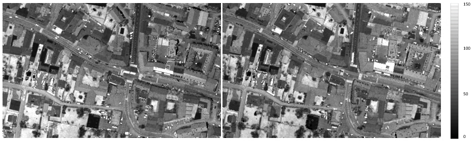
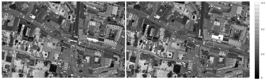
To check the results, we can e.g. create amplitude maps (Figure 2) and reflectance maps (Figure 3) for the two point clouds, before and after the radiometric calibration respectively:
Example 2: Multiple calibration constant workflow
The demo sets strip11 and strip12 are small samples of a flight strip that was captured by a RIEGL LMS-Q1560 laser scanner. This system has two laser channels (i.e. two independent laser scanners in a single body frame), which have X shaped scan pattern. strip11 originate from channel one and strip12 from channel two. Combining both data sets into a single ODM, the multiple calibration constant feature can be demonstrated. As in example 1 the necessary preprocessing steps (for the new data set strip12) are performed and both files are imported into a single ODM (strip1x.odm):
When importing multiple files into a single file, the ODM preserves the data origin in the predefined attribute FileId. In the current case, the input las file do also contain a properly set PointSourceId (namely 11 and 12), which can be easily checked using Module Info
resulting the following attribute statistics output
Hence, the attributes PointSourceId and FileId can be equally used as splitting feature for the calibration
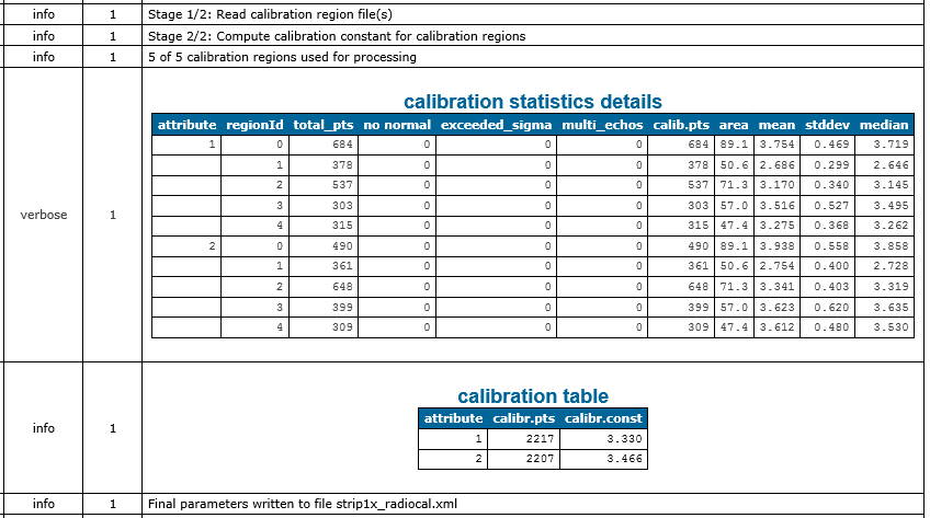
The module estimates two slightly different calibration constants for the two channels (3.330 and 3.466, also see Fig. 5). To assess if those differences are significant one can inspect the calibration details that are written as verbose messages to the opalsLog.xml
To apply the estimated calibration constants unchanged, simply used the previously created strip1x_radiocal.xml file as inParamFile parameter
In case the calibration constants should be adapted, it is possible to change the corresponding values in the parameter file or by providing an attribute-calibration-matrix as shown below:
It may occur that the overall dataset contains attribute values for which no calibration constants has been estimated or the attribute value is not set for all points. In such cases the module uses an averaged default calibration constant (derived from all given calibration constants) and outputs a corresponding warning. The following command will produce this warning since no calibration constant for attribute value '1' is defined:
It is possible to explicitly set a default calibration constant by using a single value within square brackets which also removes the aforementioned warning. E.g.
will use the calibration constant '3.3' in all situations except for points which have the attribute value '2'.
References
C. Briese, B. Höfle, H. Lehner, W. Wagner, M. Pfennigbauer, A. Ullrich: Calibration of Full-Waveform Airborne Laser Scanning Data for Object Classification in: "Proceedings of SPIE, Laser Radar Technology and Applications XIII", Vol. 6950, 2008, 69500H-69500H-8.
H. Lehner, C. Briese: Radiometric calibration of Full-Waveform Airborne Laser Scanning Data based on natural surfaces; in: "100 Years ISPRS Advancing Remote Sensing Science", XXXVIII/7B (2010), ISSN: 1682-1777; 360 - 365.
W. Wagner: Radiometric calibration of small-footprint full-waveform airborne laser scanner measurements: Basic physical concepts; in : "ISPRS Journal of Photogrammetryand Remote Sensing", Vol. 65(6), 2010, 505-513.
- Date
- 04.07.2018