

Technische Universität Wien
Orientation and Processing of Airborne Laser Scanning data
Department of Geodesy and Geoinformation - Research Groups Photogrammetry and Remote Sensing

Preprocess point clouds into the SPT partition cache (NAG format)
clfSPTPreprocress is the preprocessing step for the training workflow (clfSPTSetup -> clfSPTPreprocess -> clfSPTTrain) and the inference workflow (clfSPTPreprocess -> clfSPTInfer). It converts raw point clouds into hierachical graph structues (NAGs) on which SPT operates on. The module runs in two modes:
In training mode, it reads all tiles from the project's split folders, applies the pretransforms from the <project>.cfg file and saves them in the preprocessed folder. In inference mode, it processes individual tiles using the frozen config from the training run. Large tiles can be cut into smaller sub-tiles which will be saved alongside the input files. The core operation in both cases is the same: a raw point cloud is voxelised, partitioned into geometrically homohogenous superpoints and stored as NAG. The difference lies in where the partitioning parameters come from. At the end of every run, partition quality metrics are reported.
A NAG is a multi-level hierarchical representation of a point cloud. It represents the scene as a sequence of increasingly coarse partitions ( \(\mathcal{P}_0, \mathcal{P}_1, \dots, \mathcal{P}_I\)) along with their corresponding adjacency graphs:
knn, knn_r) is built over the \(\mathcal{P}_0\) voxels to compute local geometric features. Parallel Cut-Pursuit (pcp_regularization, pcp_cutoff) then partitions these voxels into spatially contiguous, geometrically homogeneous superpoints that respect class boundaries. As described in the SPT architecture, semantic classification is performed directly on this \(\mathcal{P}_1\) level.Each level stores its own node features (superpoints in the graph) and the adjacency graph, propagating information between superpoints. A hierarchical partition also defines a polytree structure across different levels to connect child superpoints with their parents. The adjacency graph and the polytree structure enable the model to understand the global scene and its spatial context. The number of partition levels built during preprocessing is controlled by the model parameter (default spt-2) in the .cfg file.
Because the partitioning parameters directly control graph complexity (e.g., node counts, reduction ratios) and model performance, using the preview mode is recommended to visually inspect and tune the NAG hierarchy before committing to a full run.
The training mode requires the project directory previously set up with clfSPTSetup. It reads the .cfg file from the directory and constructs the partition levels for every tile in the data/raw/{train/val/test} folders. The resulting .h5 files are saved in data/processed/{train/val/test}, which are directly loaded by clfSPTTrain. For traceability, the module copies the project's .cfg as source.cfg into each Data/Processed/{train/val/test} folder filled during a run.
When -tile is specified together with mode=train, only the given tile is processed as a quick trial run instead of the full Data/Raw/ splits. This is the recommended way to tune partitioning parameters (voxel, knn, pcp_regularization, pcp_cutoff, ground_model, ...) before committing to a full preprocessing run, which can be time-consuming on larger datasets. The processed tile and a preview_params.yaml snapshot are written to Data/Preview/<timestamp>/. Note that preview_params.yaml is informational only and cannot be used directly as a configuration file for training.
There are many ways to parametrize the preprocessing pre_transform pipeline, and finding a good setting for a new dataset is usually an iterative process. The Superpoint Transformer guidelines suggest the following target metrics for a well-balanced partition:
\[ \frac{|\mathcal{P}_0|}{|\mathcal{P}_1|} \in [30, 50] \]
\[ \frac{|\mathcal{P}_i|}{|\mathcal{P}_{i+1}|} \in [3, 10] \quad \text{for } i > 0 \]
The partition oracle represents the upper bound of segmentation accuracy (available in training mode when ground-truth labels exist) attainable with the current partition, assuming a perfect classifier. If the oracle mIoU is low, the partition is too coarse to separate semantic classes properly, and parameters (such as lowering voxel or pcp_regularization) should be adjusted before training.
At the end of each run, the module reports these partition quality metrics averaged over all processed tiles.
In inference mode, no project directory is required. Instead, the module operates directly on inputs provided via -runDir and -tile. The -runDir parameter points to either a training run directory or a standalone model bundle containing the frozen config.yaml and dataset_config.py. The preprocessing settings are loaded directly from the model's saved configuration rather than a .cfg file. This guarantees that inference uses the exact same data setup as training, preventing subtle drops in prediction quality caused by mismatched pipelines.
Optionally, a different class mapping can be used by supplying -cfg or -projectDir pointing to a project whose _config.py defines the desired classes. This project-level _config.py takes precedence over the dataset_config.py bundled in the run directory, allowing a pretrained model to be applied to a new dataset without modifying the original run files. The resulting .h5 files or, if sub-tiling is used, the <tile>_subtiles/ folder are written next to the input tile rather than into a separate project data tree.
Large airborne laser scanning (ALS) tiles often contain tens of millions of points, vastly exceeding system RAM limits during graph construction. Subtiling breaks down such massive point clouds into manageable spatial chunks that fit comfortably within hardware resource constraints.
Subtiling is strictly reserved for inference mode. For training, tiles must be prepared at a known, manageable size before clfSPTSetup without cutting through important features (e.g., vehicles, rooftops) so that each tile fits into memory as a whole. Processing a tile in one piece preserves the complete superpoint graph without artificial boundary cuts. While an overlapping buffer protects the inner core zone of a sub-tile, it still creates a hard spatial boundary along the outer buffer edge where the graph is truncated. During training, loss gradients are computed across the entire input graph. Training on sub-tiles would force the network to compute loss on artificially cut superpoints and incomplete neighborhood graphs, contaminating gradients and systematically degrading the model's ability to learn accurate object boundaries.
Processing an isolated sub-tile without surrounding context leads to classification errors near its boundaries. Boundary artifacts occur most prominently within the first ~5 meters of a cut edge, where neighborhood-based geometric features suffer from missing context. To eliminate these boundary artifacts, the bounding box of the tile is divided into a regular grid of cells with side length \(T\) (-tileSize). Along each axis, points are assigned to zone types as follows:
| Tile type | X axis | Y axis | Shape |
|---|---|---|---|
| Core tile | core zone | core zone | \((T - 2b) \times (T - 2b)\) (interior cells) |
| Edge tile | seam zone / core zone | core zone / seam zone | narrow strip \(2b \times (T - 2b)\) |
| Corner tile | seam zone | seam zone | small square \(2b \times 2b\) |
The diagram below shows a 2x2 example grid:
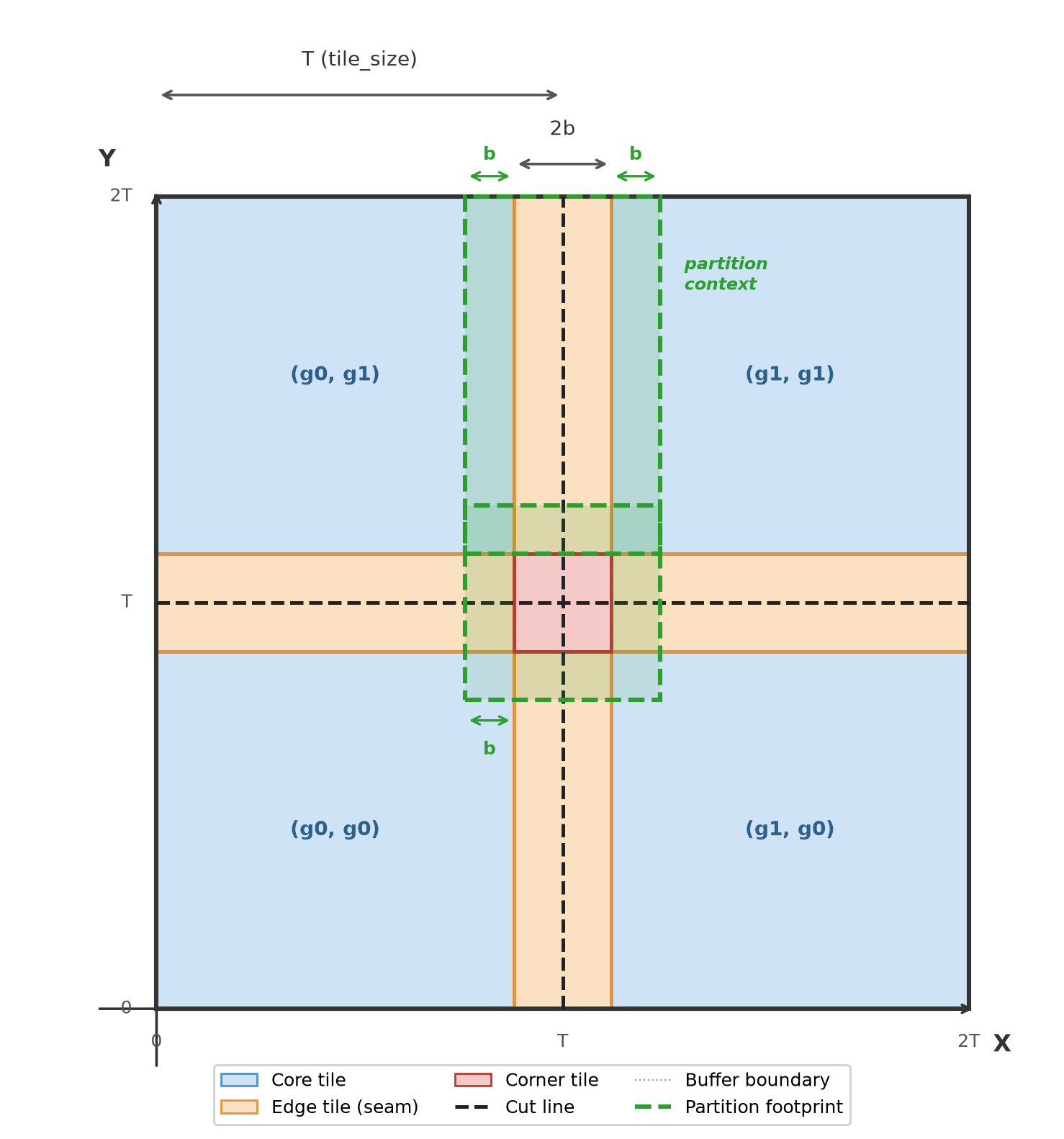
The tile size must satisfy \(T > 4b\) otherwise, the core zones collapse to zero width and an error is raised. If the tile's extent is smaller than \(T\) in one or both axes, no seam zones are generated along that axis (e.g., narrow flight strips are automatically handled as 1D strip tilings). If the entire tile fits within a single cell, no subtiling occurs, and a single NAG is written without a manifest.
When subtiling is active, sub-NAGs are stored in a <tile>_subtiles/ directory alongside a manifest.json. clfSPTPreprocess additionally writes an ESRI shapefile of the subtile footprints <stem\>_subtiles/\<stem\>_tiles.shp. The coordiante reference system is read from the source tile automatically, -epsg can be used to force a specific CRS when the source carries none or to override it. The .prj file is only written if a CRS could be determined, otherwise the shapefile is written without a projection.
The manifest records the source tile, the frozen config.yaml path, tileSize, and buffer values, as well as per-subtile metadata (filename, tile type, spatial footprint, and point count). clfSPTInfer reads this manifest directly to classify each sub-NAG.
Sub-tiles with fewer than 64 points or failed partitioning (common for thin edge/corner tiles) are skipped with a warning. Their core points remain covered by the buffer of neighboring core tiles, preventing spatial gaps.
The SPT model uses a height_above_ground feature internally, computed as part of its partition transform chain. Three ground estimation methods are available (set via ground_model in the .cfg):
Alternatively, ELEVATION_SOURCE can be set to 'opals' in the project's <project>_config.py. In this case, the model expects a precomputed NormalizedZ attribute and skips internal ground estimation entirely. For deriving the NormalizedZ attribute please take a look at AddInfo.
| train |
| infer |
| possible input | evaluates to |
|---|---|
| 1, true, yes, Boolean(True), True | Boolean(True) |
| 0, false, no, Boolean(False), False | Boolean(False) |
Always run a single-tile preview first to verify partition quality before committing to a full run:
The preview reports partition statistics and oracle metrics, the theoretical upper bound on accuracy given the partition granularity:
With -view True, the partition is also visualized interactively:
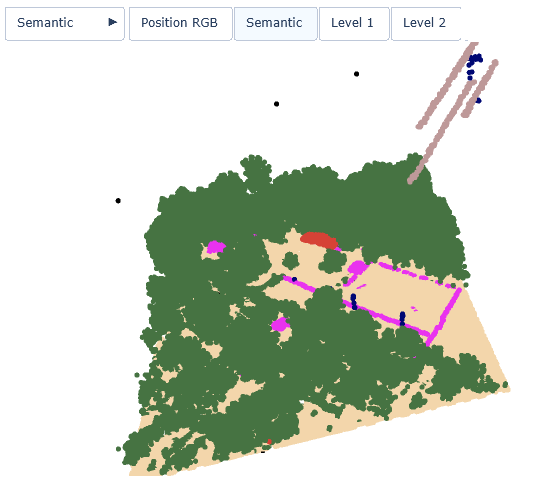 Fig. 2 Semantic classes | 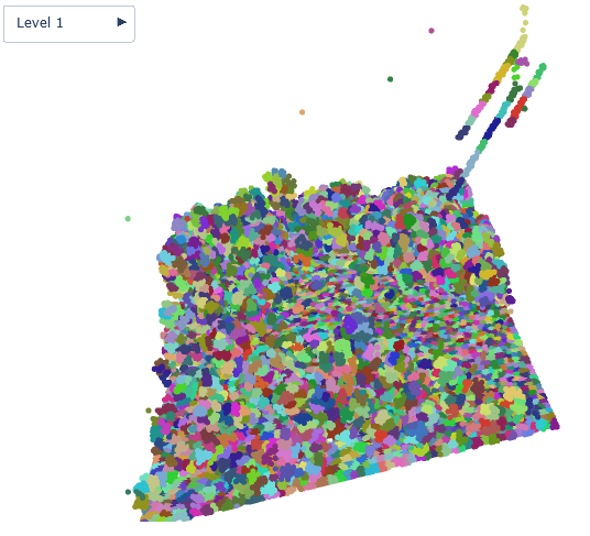 Level 1 partition | 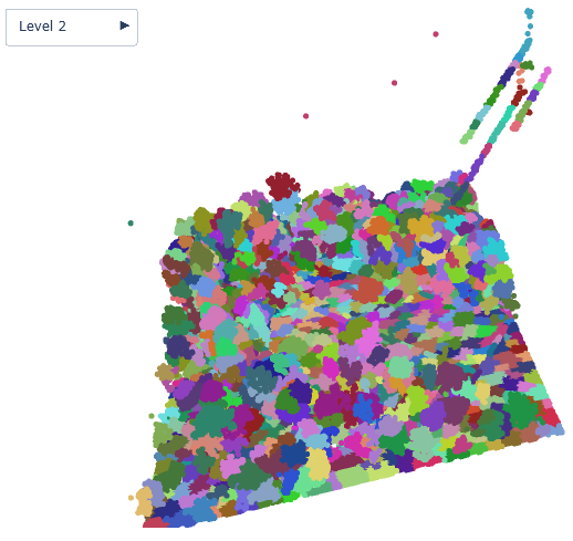 Level 2 partition |
When comparing preview vs. full preprocessing oracle values the overall oracle is averaged across all sub-tiles. Some sub-tiles cover nearly homogeneous areas (e.g. only forest), where the partition achieves near-perfect separation. These easy tiles raise the overall average compared to the single-tile preview, which may contain a more diverse class mix.
Output shows averaged oracle metrics across all tiles:
 1.8.17