

Technische Universität Wien
Orientation and Processing of Airborne Laser Scanning data
Department of Geodesy and Geoinformation - Research Groups Photogrammetry and Remote Sensing

This package provides a workflow for training and applying a Superpoint Transformer (SPT) to classify point clouds by semantic class. The four modules clfSPTSetup, clfSPTPreprocess, clfSPTTrain, and clfSPTInfer cover the full workflow from training on labelled tiles to creating a trained model and applying it to new, unlabelled data.
The integration of SPT in OPALS follows two separate workflows that share a common preprocessing step.
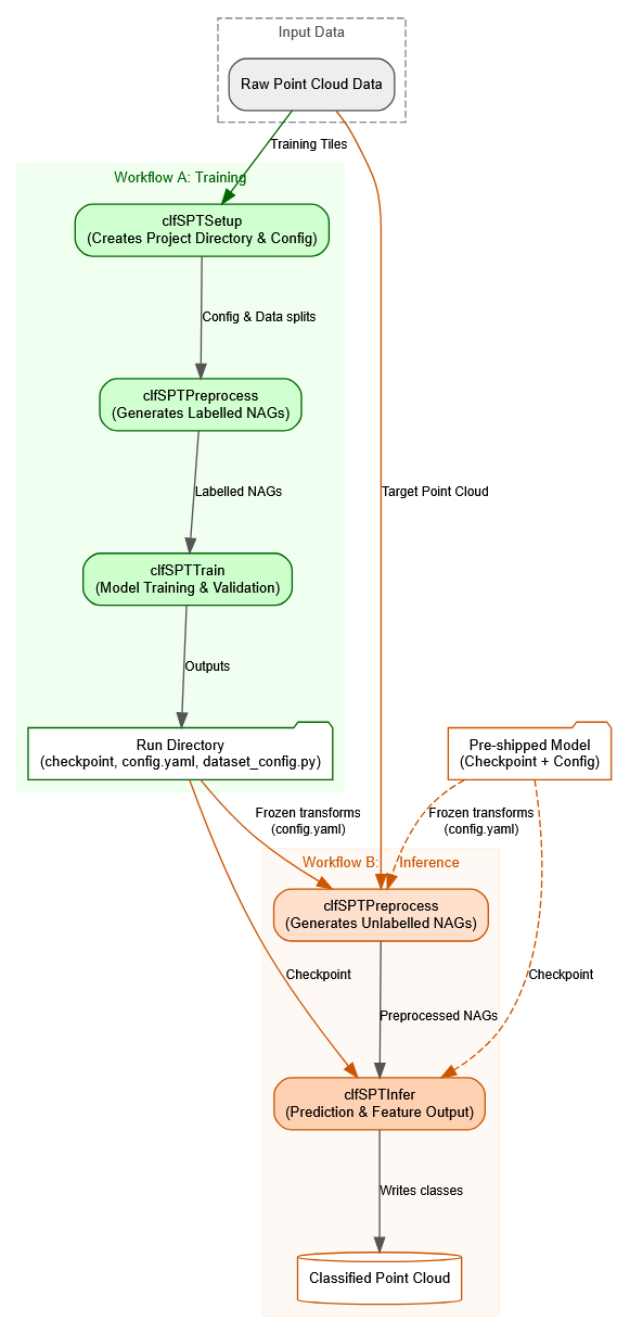
In this workflow, the model is trained on labelled point cloud data using the following scripts:
Unlike the tree-based classification (Tree Based Classification), SPT does not rely on a fixed, externally precomputed feature set. Most geometric features it uses (linearity, planarity, scattering, verticality, and elevation) are computed internally as part of the model's own partitioning pipeline (see clfSPTPreprocess) and require no separate OPALS preprocessing step.
A small number of attributes can optionally be derived beforehand with dedicated OPALS modules: NormalX/Y/Z (Module Normals) and EchoRatio (Module EchoRatio) can be computed explicitly to make them available as model features. Elevation can likewise be sourced from a precomputed NormalizedZ attribute (AddInfo) instead of SPT's internal ground estimation. See Feature detection in clfSPTSetup for the full list and how detected/available attributes are matched to model features. Non geometric features like : intensity/RGB/reflectance are picked up automatically if present.
Due to the lack of an interactive 3D point cloud editor, it is currently not possible to visually create training data within OPALS. However, several commercial and open source software packages (e.g. \href{http://www.meshlab.net/}{MeshLab}, \href{http://www.danielgm.net/cc/}{CloudCompare}, etc.) exist for this task. The labelled point cloud can then be merged back into the corresponding ODM files (or exported as LAS/LAZ with a populated classification attribute) and directly processed with clfSPTSetup.
In this workflow, a produced run directory or a pre-trained model is applied to unlabelled data:
Raw point clouds from ALS or dense image matching usually contain outliers. Their characteristics and amount differ based on the measurement principle and sensor. In ALS such outliers are often called long or short ranges, since they are obviously not reflected from either the bare Earth or from any other natural (vegetation) or artificial (buildings, power lines) target.
Any gross error distorts the geometric features computed within its vicinity. For SPT this affects the k-nearest-neighbor graph, the local geometric features (linearity, planarity, scattering, verticality) and, downstream, the Cut-Pursuit partitioning itself (see clfSPTPreprocess). Since these features drive both the superpoint partitioning and the semantic classification, outlier contamination here can degrade results more broadly than in a per-point classifier: a single gross error can corrupt the neighborhood features of many surrounding points, and if it distorts a superpoint's shape enough, it can pull that entire superpoint (and everything merged into it) toward an incorrect classification.
Practical tests have shown that classification accuracies are usually better for point clouds where outliers have been removed in advance. A detailed discussion on efficient outlier detection is omitted here, detecting isolated points (e.g. via AddInfo) and applying a coarse DTM/DSM to filter implausible heights is generally sufficient to solve this task before running clfSPTInfer.
As a prerequisite, the demo tile is imported and cut into sub-tiles of 265x200 m so that a small training set with multiple tiles can be created from a single scene.
clfSPTSetup distributes the sub-tiles into train/val/test splits and generates the project configuration. The class mapping must be defined beforehand by renaming the generic Classification attribute values to semantic labels (see Setup configuration and Setup examples for details on the interactive remapping dialog).
The per-split class distribution above illustrates why reviewing this output is worthwhile before training. Most classes (2, 5, 6, 8, 11, 14, 18, 30) keep a broadly similar share of points across train, val, and test, which is what a representative split looks like. Classes 9, 16, and 31, however, are unevenly distributed: class 9 drops from 11.3% of the train split to 3.3% in val and just 0.8% in test; class 31 similarly falls from 0.5% in train to 0.1% in val and is essentially absent from test (2 out of 348,531 points); class 16 is reduced to a single point in val and is completely absent from test.Metrics reported for class 16 on the test split are therefore not meaningful, there is nothing there to measure against. Note also that the resulting split ratio (56.4/25.8/17.7%) does not match the requested -trainRatio/-valRatio exactly, since clfSPTSetup distributes whole tiles rather than individual points, and tiles vary considerably in point count. When a class is this sparse, either merging it with a related class during the interactive class mapping, or adjusting the split ratios or tile selection to secure a few more tiles containing it, is recommended before proceeding to clfSPTPreprocess and clfSPTTrain.
Before processing the full dataset, clfSPTPreprocess can be run on a single tile with -view True to visually inspect partition quality and feature computation. See Preprocess training mode for a detailed discussion of partition parameters and oracle metric interpretation.
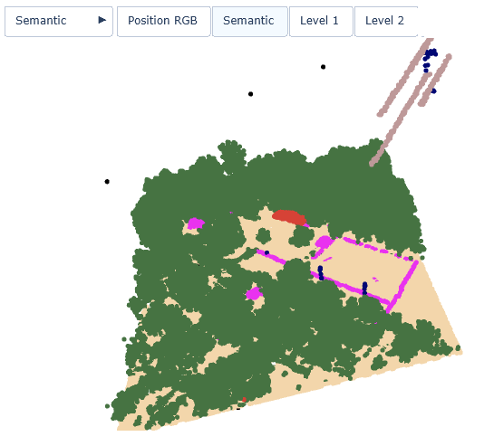 Fig. 2 Semantic classes | 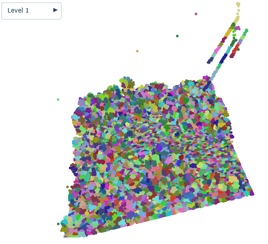 Level 1 partition |
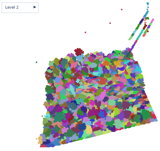 Level 2 partition | 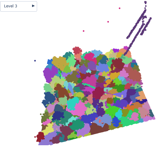 Level 3 partition |
Once the partition quality is satisfactory, all tiles are preprocessed at once. The cached NAGs are reused across multiple training runs with different hyperparameters.
clfSPTTrain reads the .cfg, trains the model for the configured number of epochs, and evaluates the best checkpoint on the test split. See Train hyperparameters for details on training parameters.
After 400 epochs, the model reaches a test mIoU of ~51.6% (OA 92.3%). Classes with abundant training points (Ground, High Vegetation, Wire - Conductor) are learned reliably, with per-class IoU above 75%. Classes with very few training samples (Groyne, Road Surface, Wall) remain close to 0% IoU â this is expected for a demo dataset of this size, where rare classes are represented by too few points/tiles to be learned robustly. The confusion matrix exported alongside the metrics identifies exactly which classes these predictions are confused with, which is the recommended next step when investigating low per-class scores (see Confusion matrix in the Train module documentation).
-sweep) to keep it fast. The results reported above (test metrics, confusion matrix) come from a full 400-epoch run using the project's default clfSPTTrain -projectDir niederrhein_project, without the -sweep override) and are not representative of what a 50-epoch test run would produce.To classify new data, the tile is first preprocessed with mode=infer using the frozen transforms from the training run, then classified with clfSPTInfer. -tileSize 0 disables sub-tiling. See Infer examples for details on model loading and output handling.
Running inference on the full niederrhein.odm tile (1.9M points) as a single, unsplit NAG (-tileSize 0) versus splitting it into 200 m sub-tiles (-tileSize 200) with a 10 m buffer produces markedly different results, both in processing time and prediction quality: | | No sub-tiling (-tileSize 0) | Sub-tiling (-tileSize 200) |
Sub-tiling is not only substantially faster than building one very large graph over the entire point cloud at once but also produces clearly better predictions across nearly every class:
 1.8.17