Technische Universität Wien
Orientation and Processing of Airborne Laser Scanning data
Department of Geodesy and Geoinformation - Research Groups Photogrammetry and Remote Sensing
Airborne Laser Scanning is a widely used technique for obtaining the geometry of the Earth's surface. Apart from geometric information, ALS systems can provide additional information about the recorded signal strength of each echo. In order to utilize this information for the study of the backscatter characteristic of the sensed surface, radiometric calibration is essential. Whereas relative radiometric calibration tries to minimise radiometric differences within a strip and its neighbouring strips, absolute radiometric calibration aims at providing quantities which do not depend on mission parameters but are only related to target properties. This is achieved by using radiometric in-situ measurements acting as control elements. For more information on the principle of radiometric calibration, please refer to documentation of the opalsRadioCal module and the related literature.
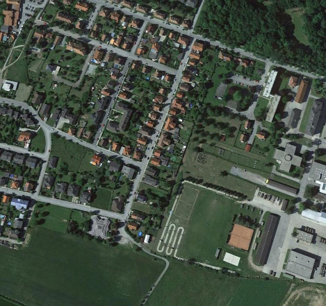
The ALS data that are used for the present use case where obtained by RIEGL Laser Measurement Systems GmbH with the laser scanner RIEGL LMS-Q680i operating at the wavelength of 1550 nm. This instrument gives the opportunity of full waveform analysis, something that is required for performing radiometric calibration. The flight was performed on the 22nd of September, 2011 and the median point density (last echo) was 11.8 points/m2. The study area is part of the town of Horn in Lower Austria, as shown in Figure 1.
Next to the ALS data acquisition, in-situ radiometric field measurements of reference surfaces were realised on the 5th December, 2011 in order to allow an absolute radiometric calibration. For that purpose, different reflecting surface types were chosen, although in the present subset of data only one of these areas is included. All areas were measured multiple times (on slightly different locations) at zero angle of incidence (observation of the surface in normal direction) and the resulting median was selected as representative reflectivity value. For the following processing it is assumed that the reflectance of these reference surfaces follows the rule of Lambert. These measurements were performed with two RIEGL reflectometer instruments.
All the necessary data as well as .bat (Windows), .sh (Linux) files and the Python script, that are going to be mentioned later on, can be downloaded as a zip folder from the OPALS download page. After the download, extract the data to the directory of your choice.
The processing of the available ALS data is divided into four different phases. In the sections that follow, there is a short description of the modules that are used during each phase as well as some comments on the results (if applicable). The corresponding code is also provided, both in the form of commandline executables and in Python (at the end of the page).
The first phase of this use case consists of the preparation of the data and the calculation of a mean calibration constant for each one of the two point clouds. This can be achieved by running the following sequence of commands for each strip (%1 should be replaced by the desired filename without extension) or simplify the run Part_1_Calculation_CalCon.bat|.sh in the OPALS Shell.
In this first phase, the two .laz files as well as the trajectory file (110922_HORN_Q680i.txt) are initially imported into the ODM. The latter is used for the extraction and storage of the trajectory information BeamVector, BeamVectorSCS, Range and ScanAngle (see parameter -storeBeamInfo in the opalsImport module), which is going to be used later on for the determination of the incidence angle of each pulse. For the same purpose, the surface normals information for each LiDAR echo is also computed, by running the opalsNormals module. In order to have a robust estimation, the number of neighbours is set to 8 in a search radius of 5 meters.
What follows next is the first use of the opalsRadioCal module, which aims at the calculation of the calibration constant. For that, the .wnp file is used, which contains the coordinates of the natural reference targets where reflectance measurements took place. In addition, the reflectivity file (calRegionHorn_reflectivity.txt) is required, in which the reflectance values of the corresponding targets can be found (In is possible to store the calibration polygons and the corresponding reflectivity values within a single shape file, as it can be found in calRegionHorn.shp. See also Module RadioCal for further details). These reflectance values refer to a specific wavelength that was used for obtaining the data (1550 nm in this use case) and to different incidence angles from 0 to 90 degrees. The following command estimated a common calibration constant for both strips.
The optional parameter outFile creates an additional ODM file (calRegions.odm in this case), that can be further used to analyze the distribution of the estimated calibration constants within the calibration regions.
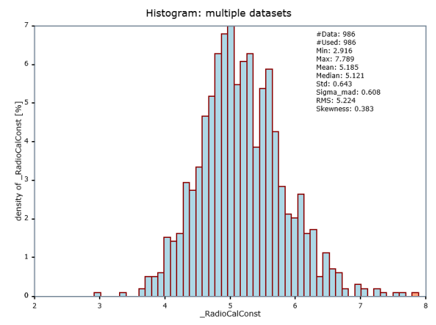
Therefore, opalsHisto module is used, having as attribute the previously calculated calibration constant (_RadioCalConst). The most robust estimator here is the median and therefore we consider from now on the median value 5.12 as the calibration constant for both strips, as also returned by the previous opalsRadioCal run. The histogram as well as the statistics of the calibration constants for both strips can be seen in Figure 2:
During the second phase, the formerly computed calibration constant is applied to both strips in order to calculate the calibrated radiometric values for each echo, by running the following command (or calling the Part_2_Application_CalCon.bat|.sh in the OPALS Shell as before):
After the second run of the opalsRadioCal module, the new radiometric attributes CrossSection, _IncidenceAngle, Reflectance, _Gamma, _Sigma, which fully describe the characteristics of the observed surface, are added to the ODM.
In the third phase of this use case, some raster colour maps are created. To produce all of the maps at once, just call Part_3_Maps.bat|.sh for each of the point clouds (filename without extension) or alternatively run the command sequence below:
Using the opalsGrid module and the corresponding attribute every time, the rasters of the amplitude (before the calibration, as it was derived from the Gaussian decomposition of the full-waveforms), the reflectance (after the calibration) and the gamma for each LiDAR echo are created. The gridsize is set to 0.25, so that all the possible details are maintained. In addition, to create a colour map, the opalsZColor module is then used. The scale was set each time so that the visualisation is clear. The left picture corresponds to the first strip (680_110922_095526.laz) and the right one to the second strip (680_110922_095947.laz) in both figures.
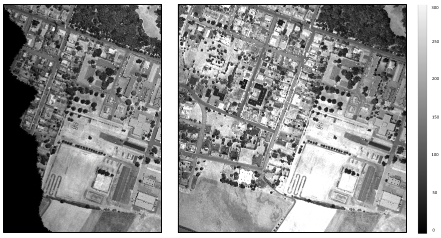
680_110922_095526.laz and right: 680_110922_095947.laz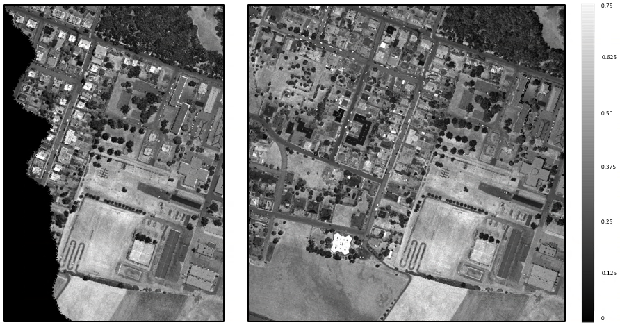
680_110922_095526.laz and right: 680_110922_095947.lazIn the amplitude maps, somebody can easily distinguish difference in the amplitude values, since it depends on a number of factors like the range, angle of incidence, surface characteristics, atmosphere etc. However, the effects of these factors have been eliminated by performing the radiometry calibration and therefore these previous difference do not appear anymore in the reflectance maps. In this way, it is possible to compare strips of different flights and/or different time periods.
The last step is to perform a radiometry check between the two strips. In order to get some insight into the quality of the performed radiometric calibration, the strip differences in the amplitude, reflectance and gamma are going to be derived. It is expected to have considerable differences before the calibration (amplitude differences) and much smaller reflectance and gamma differences between the two strips after the calibration. The script Part_4_Radiometry_Check.bat|.sh can be called and followed by both filenames this time or just run the commands below:
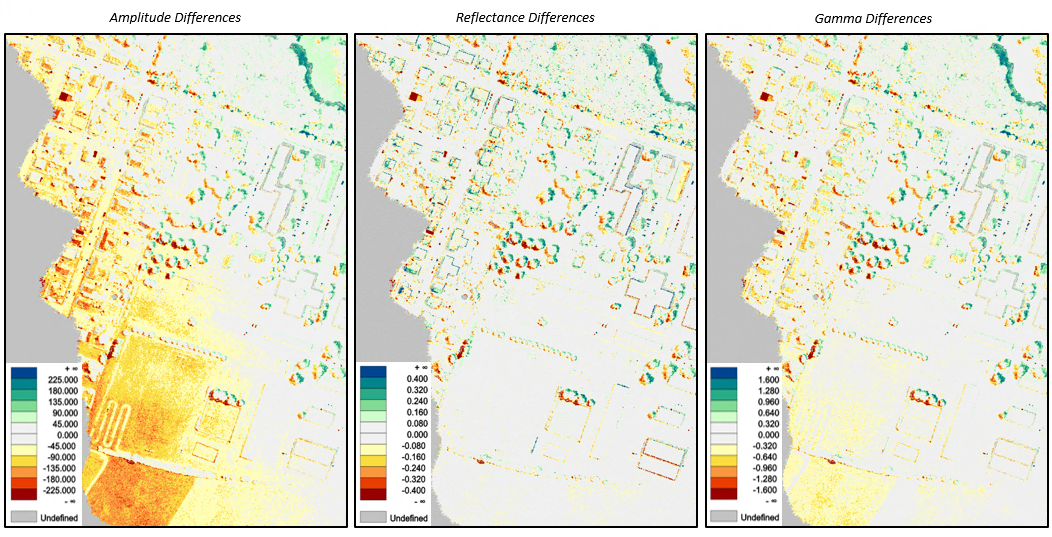
From the results shown in Figure 5, it is observed that the highest differences appear indeed in the amplitude map. That is reasonable since the effects of the influencing factors are different in each strip depending on the conditions of the flight, the atmosphere etc. On the other hand, observing the reflectance and gamma maps, it is concluded that the point clouds have become quite homogeneous after the radiometric calibration and thus they can now be used in combination with each other.
The following Python script includes four different functions that correspond to the four different phases, as described above. It is created such that the output of the one function (phase) becomes the input for the next one. It can be run both through PyScripter, which is included in the OPALS package, and in the OPALS Shell, when converted to a .py file.
Wagner, W. (2010). Radiometric calibration of small-footprint full-waveform airborne laser scanner measurements: Basic physical concepts. ISPRS Journal of Photogrammetry and Remote Sensing, 65(6), 505-513. doi:10.1016/j.isprsjprs.2010.06.007
Briese, C., Pfennigbauer, M., Lehner, H., Ullrich, A., Wagner, W., & Pfeifer, N. (2012). Radiometric Calibration Of Multi-Wavelength Airborne Laser Scanning Data. ISPRS Ann. Photogramm. Remote Sens. Spatial Inf. Sci. ISPRS Annals of Photogrammetry, Remote Sensing and Spatial Information Sciences, I-7, 335-340. doi:10.5194/isprsannals-i-7-335-2012
 1.8.17