Technische Universität Wien
Orientation and Processing of Airborne Laser Scanning data
Department of Geodesy and Geoinformation - Research Groups Photogrammetry and Remote Sensing
Performs convolutional filtering operations on a raster image.
In the case of convolutional filtering, the filter kernel (parameter kernel, i.e. a raster image) is superimposed on the input raster (parameter inFile), and corresponding pixel values are multiplied and summed up. This sum-product value is the output value of the respective pixel. The kernel is shifted along the whole image, and convolution operation is repeated for each input raster pixel. The resulting output raster (parameter outFile) is stored in GDAL supported data format (parameter oFormat). The input and output raster structure is identical. However, the output raster may be restricted to a subset of the input rasters domain (parameter limit). Please note, that this feature is not yet implemented.
In general, the convolution filter requires a complete matrix of input pixels to be superimposed with the kernel matrix. This entails that pixel values beyond the image border have to be provided in order to process the edge pixels correctly. The following parameters are offered to estimate pixel values beyond the border:
In case there are void data pixels in the current neighbourhood, the sum-product can either be calculated by omitting these void pixels or the respective output pixel itself may be set to void (parameter ignoreNoData). Please note, that void pixels are generated if all image pixels within the current kernel area are invalid (i.e. nodata). Additionally, the marker indicating data voids in the output raster can be set by the user (parameter noData). Finally, the pixel-wise sum-product may be stored as is, or otherwise normalized, i.e. divided by the sum of the kernel values (parameter normalize).
The kernel matrix constitutes the main input for Module Convolution besides the input raster itself. Kernels can either be selected form a list of pre-defined kernels or specified explicitly by the user. The following syntax applies:
The first two (AVERAGE, GAUSSIAN) are pre-defined kernels requiring only the kernel size (number of columns/rows). The Gaussian kernel additionally requires the standard deviation of the gauss function (SIGMA).
Arbitrary user-defined kernels can be read from an existing raster file (FROMFILE) in GDAL supported data format. The georeferencing of the raster file is ignored, but the kernel matrix as read from file is superimposed to the image matrix 1:1. Note, that void pixels are not allowed in the kernel matrix. Finally, the kernel matrix (KM) can also be specified manually by providing both the size of the kernel (m..columns,n..rows) and the matrix elements themselves (elements in row major order, i.e.: k11 k12 ... knm)
\( \mathbf{KM} = \begin{pmatrix}k_{11} & k_{12} & k_{13} & ... & k_{1m} \\ k_{21} & k_{22} & k_{23} & ... & k_{2m} \\ ... & ... & ... & ... & ... \\ k_{n1} & k_{n2} & k_{n3} & ... & k_{nm} \end{pmatrix} \),
Please note, that the rows and columns count both must be odd, for pre-defined as well as for user-defined kernels. The kernel matrix values are of float type.
A simple 5x5 average yielding the kernel matrix:
\( \mathbf{KM} = \begin{pmatrix} 1 & 1 & 1 & 1 & 1 \\ 1 & 1 & 1 & 1 & 1 \\ 1 & 1 & 1 & 1 & 1 \\ 1 & 1 & 1 & 1 & 1 \\ 1 & 1 & 1 & 1 & 1 \end{pmatrix} \),
An asymmetric 5 columns x 3 rows gaussian filter with a standard deviation of 0.75. The resulting kernel matrix is:
\( \mathbf{KM} = \begin{pmatrix} 0.0033 & 0.0478 & 0.1163 & 0.0478 & 0.0033 \\ 0.0081 & 0.1163 & 0.2829 & 0.1163 & 0.0081 \\ 0.0033 & 0.0478 & 0.1163 & 0.0478 & 0.0033 \\ \end{pmatrix} \),
A user defined 3x3 kernel. Note, the values are entered in row major order starting from the upper left corner, thus, the corresponding kernel matrix is:
\( \mathbf{KM} = \begin{pmatrix} 1.00 & 0.00 & 1.00\\ 0.00 & 1.00 & 0.00\\ 1.00 & 0.00 & 1.00\\ \end{pmatrix} \),
Finally, an example for reading the kernel matrix from a raster file (Tiff).
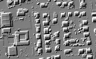
The data used in the following example are located in the $OPALS_ROOT/demo/ directory. For the strip 21 (contained in the demo directory) the following commands are required to obtain DSM model:
As a result, a grid file strip21.tif in GeoTiff format is created. A hill shading is shown in Figure 1.
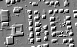
In this example smoothing is performed by applying a 5x5 Gaussian filter with a sigma value of 2.0.
A hill shading of the resulting model is shown in Figure 2.
In this example smoothing is performed via a user-defined 3x3 filter. The calculated filter value is normalized with the number of non-noData values covered by the kernel.
In this example a user-defined 3x3 filter in GDAL format is created and applied to a raster image.
It takes several steps to produce a filter kernel file in GDAL raster image format. One possible solution is as follows: Use a text editor, to create a xyz format ASCII file (e.g. conic_3x3.xyz in your working directory, containing the filter kernel coefficients. (For format definition see: Module Import).
conic_3x3.xyz should look like this:
(Use tab or blanks between numeric values.) First two coloumns denote the kernel matrix indices (columns and rows) while the third coloumn contains the kernel coefficients.
The first line corresspond to the top left corner of the 3x3 filter kernel (column 1, row 1), and the following lines correspond to the subsequent kernel coefficient (row major order). The last line corresponds to the bottom right corner of the filter kernel (column 3, row 99). The following commands are required to obtain the kernel in raster file format:
The filter kernel file conic_3x3.tif in GeoTiff format is created and can, now, be used for convoluting a raster file:
 1.8.17