Technische Universität Wien
Orientation and Processing of Airborne Laser Scanning data
Department of Geodesy and Geoinformation - Research Groups Photogrammetry and Remote Sensing
Airborne Laser Scanning delivers not only point positions, but also various point attributes related to the properties of the measured echoes. Additionally, user-generated attributes can also be created, describing texture, structure and radiometric properties of each point and their neighbourhoods. Visual representation of these attributes is essential for effectively using them in point cloud filtering, classification and analysis. Traditional GIS software can visualize rasters and vectors based on their attributes, but point cloud visualization software typically only handle the pre-defined attributes available in the data format they are using (mostly .las). This means other user-generated attributes are not possible to directly visualize through colouring of the points themselves. OpalsColorize exploits the built-in Red, Green, Blue attributes of both the OPALS .odm and the ISPRS .las file for visualization, and allows re-scaling of attribute values to these color attributes, using either pre-defined palettes or RGB visualization.
This use case is based on the data of the Radiometric calibration of full waveform ALS data, Horn, Austria use case. The processing starts with the two .odm files output after the Radiometric Calibration use case is complete. We start with the two .odm files created at the end of the RadioCal Use case. These are two overlapping full-waveform airborne LIDAR flight strips with imported trajectory data, beam vectors, and calibrated reflectance.
First we run OpalsInfo on the two strips to see what attributes they hold
The opalsinfo output is as follows:
Filename
c:\Data\opalscolorize_use_case\dev_colorize_use_case\680_110922_095526.odm
Type    odm
SpatialReference        PROJCS["WGS 84 / UTM zone 33N",GEOGCS["WGS
84",DATUM["WGS_1984",SPHEROID["WGS
84",6378137,298.257223563,AUTHORITY["EPSG","7030"]],AUTHORITY["EPSG","6326"]],PRIMEM["Greenwich",0,AUTHORITY["EPSG","8901"]],UNIT["degree",0.0174532925199433,AUTHORITY["EPSG","9122"]],AUTHORITY["EPSG","4326"]],PROJECTION["Transverse_Mercator"],PARAMETER["latitude_of_origin",0],PARAMETER["central_meridian",15],PARAMETER["scale_factor",0.9996],PARAMETER["false_easting",500000],PARAMETER["false_northing",0],UNIT["metre",1,AUTHORITY["EPSG","9001"]],AXIS["Easting",EAST],AXIS["Northing",NORTH],AUTHORITY["EPSG","32633"]]
Point Count     1095464
Line Count      0
Polygon Count   0
Minimum X-Y-Z     548355.271 5389534.000   321.017
Maximum X-Y-Z     548701.000 5390034.000   415.035
Point density   0.61
Attribute       type    count   min     max     mean    sigma
Amplitude       float   1095464 10.000  23874.000       133.781 81.664
EchoNumber      uint8   1095464 1       7       1.210 0.530
NrOfEchos       uint8   1095464 1       7       1.419 0.765
ClassificationFlags     uint8    1095464 0       0 0.000   0.000
ScanDirection   bool 1095464 0       0       0.000   0.000
EdgeOfFlightLine        bool 1095464 0       0       0.000 0.000
Classification  uint8   1095464 0       0       0.000 0.000
ScanAngle       float   1095464 0.022   0.557   0.328   0.133
UserData        uint8   1095464 0       0       0.000 0.000
PointSourceId   uint16  1095464 0       0       0.000 0.000
GPSTime double  1095464 381375.874      381385.716 381380.482      2.407
EchoWidth       float   1095464 3.000   26.700  4.618   0.650
BeamVectorX     float   1095464 -388.474        7.684 -187.519        86.269
BeamVectorY     float   1095464 -142.926        -23.125 -74.467 24.795
BeamVectorZ     float   1095464 -598.542        -507.674 -559.442
5.714
_BeamVectorSCSX float   1095464 -1.214  1.076   -0.120  0.525
_BeamVectorSCSY float   1095464 12.581  343.868 195.275 85.006
_BeamVectorSCSZ float   1095464 516.645 595.460 562.435 11.292
Range   float   1095464 526.293 695.386 600.629 31.914
Id      int64   1095464 6442450944      1125919234205058 649683261817435.370
379675618954346.500
FileId  uint16   1095464 1       1       1.000   0.000
LayerId uint16   1095464 0       0       0.000   0.000
WinputCode      uint16   1095464 30      30      30.000 0.000
StructNr        uint16   1095464 0       0       0.000 0.000
NormalX float   918990  -1.000  1.000   0.060   0.403
NormalY float   918990  -1.000  1.000   0.028   0.411
NormalZ float   918990  0.000   1.000   0.698   0.421
NormalSigma0    float   918990  0.000   0.994   0.079   0.100
NormalEstimationMethod  uint8    918990  0       0 0.000   0.000
CrossSection    float   0       ---     ---     ---     ---
_IncidenceAngle float   1095464 0.000   84.999  13.383  15.064
Reflectance     float   1095464 0.012   56.456  0.318   0.260
_Gamma  float   1095464 0.048   225.826 1.129   0.699
_Sigma  float   0       ---     ---     ---     ---
Index statistics
geometries      dim     type    depth   node count      leaf count
tile size
min #owl        max #owl        mean #owl       stddev #owl
Points  2       tile    1       25      21      107.250 1361 106195
52164.952
36028.082
So the file has approximately 1000000 points with
Theoretically, all the numeric attributes can be visualized using OpalsColorize on a point basis.
We run OpalsInfo on the other file as well:
The output is the same, but with approximately 2000000 points.
Filename
c:\Data\opalscolorize_use_case\dev_colorize_use_case\680_110922_095947.odm
Type    odm
SpatialReference        PROJCS["WGS 84 / UTM zone 33N",GEOGCS["WGS
84",DATUM["WGS_1984",SPHEROID["WGS
84",6378137,298.257223563,AUTHORITY["EPSG","7030"]],AUTHORITY["EPSG","6326"]],PRIMEM["Greenwich",0,AUTHORITY["EPSG","8901"]],UNIT["degree",0.0174532925199433,AUTHORITY["EPSG","9122"]],AUTHORITY["EPSG","4326"]],PROJECTION["Transverse_Mercator"],PARAMETER["latitude_of_origin",0],PARAMETER["central_meridian",15],PARAMETER["scale_factor",0.9996],PARAMETER["false_easting",500000],PARAMETER["false_northing",0],UNIT["metre",1,AUTHORITY["EPSG","9001"]],AXIS["Easting",EAST],AXIS["Northing",NORTH],AUTHORITY["EPSG","32633"]]
Point Count     2000660
Line Count      0
Polygon Count   0
Minimum X-Y-Z     548201.001 5389534.000   319.819
Maximum X-Y-Z     548701.000 5390034.000   420.567
Point density   0.56
Attribute       type    count   min     max     mean    sigma
Amplitude       float   2000660 10.000  65517.000       172.725 119.138
EchoNumber      uint8    2000660 1       7       1.158 0.455
NrOfEchos       uint8    2000660 1       7       1.318 0.664
ClassificationFlags     uint8    2000660 0       0 0.000   0.000
ScanDirection   bool 2000660 0       0       0.000   0.000
EdgeOfFlightLine        bool 2000660 0       0       0.000 0.000
Classification  uint8    2000660 0       0       0.000 0.000
ScanAngle       float   2000660 -0.522  0.558   0.040   0.251
UserData        uint8    2000660 0       0       0.000 0.000
PointSourceId   uint16   2000660 0       0       0.000 0.000
GPSTime double  2000660 381607.216      381618.474 381613.123      2.403
EchoWidth       float   2000660 1.600   28.000  4.642   0.608
BeamVectorX     float   2000660 -281.645        298.890 15.565 127.223
BeamVectorY     float   2000660 -138.602        164.437 17.263 62.536
BeamVectorZ     float   2000660 -583.272        -484.437 -544.106
4.923
_BeamVectorSCSX float   2000660 -1.136  3.138   0.933   0.904
_BeamVectorSCSY float   2000660 -313.871        342.940 22.844 142.387
_BeamVectorSCSZ float   2000660 484.980 585.881 543.968 5.719
Range   float   2000660 485.176 648.505 562.468 18.485
Id      int64   2000660 2147483648      1125919234260358 636357768932269.250
339547697230284.690
FileId  uint16   2000660 1       1       1.000   0.000
LayerId uint16   2000660 0       0       0.000   0.000
WinputCode      uint16   2000660 30      30      30.000 0.000
StructNr        uint16   2000660 0       0       0.000 0.000
NormalX float   1745996 -1.000  1.000   -0.001  0.376
NormalY float   1745996 -1.000  1.000   0.005   0.370
NormalZ float   1745996 0.000   1.000   0.761   0.378
NormalSigma0    float   1745996 0.000   1.266   0.072   0.096
NormalEstimationMethod  uint8    1745996 0       0 0.000   0.000
CrossSection    float   0       ---     ---     ---     ---
_IncidenceAngle float   2000660 0.000   84.999  9.830   12.065
Reflectance     float   2000660 0.012   146.687 0.334   0.245
_Gamma  float   2000660 0.050   586.747 1.268   0.892
_Sigma  float   0       ---     ---     ---     ---
Index statistics
geometries      dim     type    depth   node count      leaf count
tile size
min #owl        max #owl        mean #owl       stddev #owl
Points  2       tile    1       25      25      128.000 4851 139210
80026.400
46672.537
We merge the two files to one single data file for easier handling, by importing the two .odms to a single .odm
In this case, OpalsImport retains all the attributes of the two source files. We check this in OpalsInfo:
The result is as follows:
Filename c:\Data\opalscolorize_use_case\dev_colorize_use_case\points.odm
Type    odm
SpatialReference        PROJCS["WGS 84 / UTM zone 33N",GEOGCS["WGS
84",DATUM["WGS_1984",SPHEROID["WGS
84",6378137,298.257223563,AUTHORITY["EPSG","7030"]],AUTHORITY["EPSG","6326"]],PRIMEM["Greenwich",0,AUTHORITY["EPSG","8901"]],UNIT["degree",0.0174532925199433,AUTHORITY["EPSG","9122"]],AUTHORITY["EPSG","4326"]],PROJECTION["Transverse_Mercator"],PARAMETER["latitude_of_origin",0],PARAMETER["central_meridian",15],PARAMETER["scale_factor",0.9996],PARAMETER["false_easting",500000],PARAMETER["false_northing",0],UNIT["metre",1,AUTHORITY["EPSG","9001"]],AXIS["Easting",EAST],AXIS["Northing",NORTH],AUTHORITY["EPSG","32633"]]
Point Count     3096124
Line Count      0
Polygon Count   0
Minimum X-Y-Z     548201.001 5389534.000   319.819
Maximum X-Y-Z     548701.000 5390034.000   420.567
Point density   1.15
Attribute       type    count   min     max     mean    sigma
Amplitude       float   3096124 10.000  65517.000       158.946 108.987
EchoNumber      uint8    3096124 1       7       1.176 0.483
NrOfEchos       uint8    3096124 1       7       1.354 0.703
ClassificationFlags     uint8    3096124 0       0 0.000   0.000
ScanDirection   bool 3096124 0       0       0.000   0.000
EdgeOfFlightLine        bool 3096124 0       0       0.000 0.000
Classification  uint8    3096124 0       0       0.000 0.000
ScanAngle       float   3096124 -0.522  0.558   0.142   0.257
UserData        uint8    3096124 0       0       0.000 0.000
PointSourceId   uint16   3096124 0       0       0.000 0.000
GPSTime double  3096124 381375.874      381618.474 381530.811      111.264
EchoWidth       float   3096124 1.600   28.000  4.634   0.624
BeamVectorX     float   3096124 -388.474        298.890 -56.290 150.072
BeamVectorY     float   3096124 -142.926        164.437 -15.193 68.325
BeamVectorZ     float   3096124 -598.542        -484.437 -549.532
8.999
_BeamVectorSCSX float   3096124 -1.214  3.138   0.560   0.938
_BeamVectorSCSY float   3096124 -313.871        367.928 83.854 149.850
_BeamVectorSCSZ float   3096124 484.980 595.460 550.502 12.009
Range   float   3096124 485.176 695.386 575.970 30.234
Id      int64   3096124 2147483648      1407372736120332 642031292303116.750
360738370783687.810
FileId  uint16   3096124 1       2       1.646   0.478
LayerId uint16   3096124 0       0       0.000   0.000
WinputCode      uint16   3096124 30      30      30.000 0.000
StructNr        uint16   3096124 0       0       0.000 0.000
NormalX float   2664986 -1.000  1.000   0.020   0.386
NormalY float   2664986 -1.000  1.000   0.013   0.385
NormalZ float   2664986 0.000   1.000   0.739   0.394
NormalSigma0    float   2664986 0.000   1.142   0.074   0.097
NormalEstimationMethod  uint8    2664986 0       0 0.000   0.000
CrossSection    float   0       ---     ---     ---     ---
_IncidenceAngle float   3096124 0.000   84.999  11.087  13.313
Reflectance     float   3096124 0.012   146.687 0.328   0.250
_Gamma  float   3096124 0.048   586.747 1.219   0.832
_Sigma  float   0       ---     ---     ---     ---
Index statistics
geometries      dim     type    depth   node count      leaf count
tile size
min #owl        max #owl        mean #owl       stddev #owl
Points  2       tile    1       25      25      125.500 13756 287781
123844.960
79551.495
This file now has about 3100000 points, with all the original attributes. The attribute FileId refers to the original source files, and is "1" and "2" respectively. We can check this using a basic OpalsColorize command:
OpalsColorize edits the Red, Green and Blue attributes of an .odm file to create colour outputs based on the values of other attributes. This means that the selected attribute values are rescaled to match the range of the RGB attribute. The default case is that only an .odm is generated, with new attributes. However, if additionally an output .las file is specified, then such a file is also generated, with the color written to the R,G,B attributes of the .las file. For this command, OpalsColorize gives the following output
16:35:13 info: Running opalsColorize ...
16:35:13 info: Index statistics
geometries      dim     type    depth   node count      leaf count
tile size
min #owl        max #owl        mean #owl       stddev #owl
Points  2       tile    1       25      25      125.500 13756 287781
123844.960
79551.495

16:35:13 info: Stage 1/1: Classifying data
100%16:35:24 info: Class No.    FileId : Count
    0            BG : 0
    1       underfl : 0
    2         1.000 : 1095464
    3         1.004 : 0
    4         1.008 : 0
...
...
  253         1.992 : 0
  254         1.996 : 0
  255         2.000 : 2000660


16:35:24 info: Running opalsColorize took: 00:00:11
This means that we are using the default palette with 255 colour steps, which is $OPALS_ROOT$/addons/pal/standardPal.xml . This palette runs from green to brown, in our case this means that points with FileId == 1 will be coloured green, while points with FileId == 2 will be coloured brown. By opening the resulting .las point cloud in a point cloud viewer (eg. FugroViewer, CloudCompare), the output point cloud can be checked visually in planar, profile or 3D perspective view.
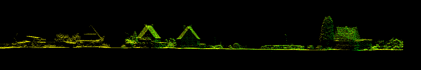
Additionally, a basic .svg graphic file legend is generated with attribute values and their respective colouring.
The Echo width values have the following distribution (from the OpalsInfo output):
EchoWidth float 3096124 1.600 28.000 4.634 0.624
What if we want a different color scheme? We apply a different palette from the folder $OPALS_ROOT$/addons/pal/ or our own user-defined .xml palette files. E.g.
this will result in points with FileId == 1 coloured red, and points with FileId == 2 coloured blue. Please note that applying OpalsColorize on the same output file repeatedly will overwrite the Red, Green and Blue values in the file.
Now we visualize another point attribute: Echo Width.
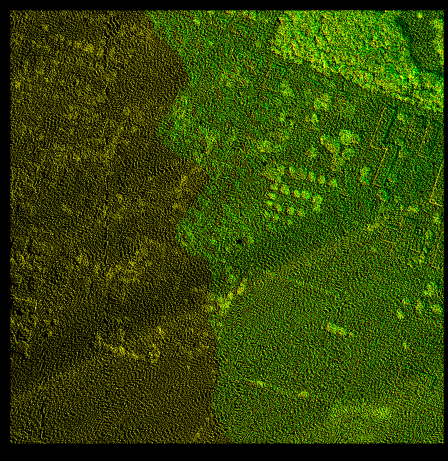
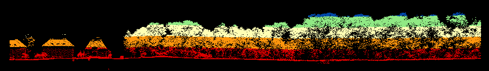
In this case the minimum and maximum value range of Echo Width are automatically mapped to the palette nodes with a linear stretch. The minimum is 0, the maximum is 28, and the resulting legend can be viewed as the file points_EchoWidth_EchoWidth_Legend.svg. However, this visualization is not informative as nearly all points have very similar shades of green. In order to get a better overview of the EchoWidth distribution, a linear scaling can be applied, excluding points above and below a certain limit, e.g. 1 Sigma from the mean. This is 4.636 ± 0.624, so 4 and 5.5 are reasonable limits that we can expect to contain most of the data. These can be applied to coloring with the -ScalePal parameter. Here we use another palette in order to get a wider colour range:
This results in low echo width points becoming red, medium echo width points orange, and high echo width points green. A more detailed visualization can be achieved by setting a higher number of classes using the parameter -nclasses
Or even better, steps in the palette can be introduced manually, eg. to enhance specific intervals. For this, we first calculate a histogram of Echo Width, within the already established upper and lower limits, to avoid outliers.
Based on the histogram, we use the following intervals: 4,4.1,4.2,4.5,4.7,5,5.5,6 . We enter these steps into the Scalepal parameter as before
On this .las dataset the colours of the palette correspond exactly to the specified intervals and therefore allow quantitative interpretation of echo width. Alternatively, histogram equalization can be used for generating a visually more appealing output that enhances the heterogeneity of the data
Normalized height is another important attribute for point-level visualization. For calculating normalized height, first we generate a very basic Digital Terrain Model (DTM) by taking the second lowest point in every 5 m cell, then smoothing with a minimum filter
Then we use this grid to calculate normalized height as a new attribute, and check its typical values with opalshisto
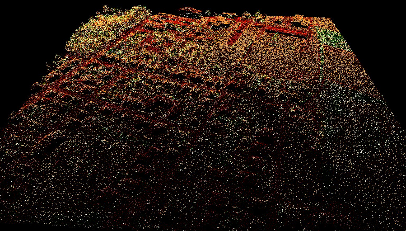
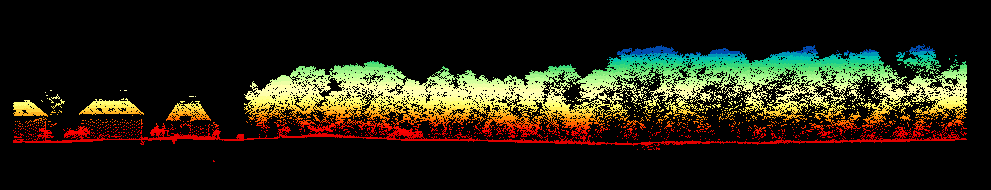
NormalizedZ varies between 0 and 25 m, with a some rare points having negative values. We visualize NormalizedZ with opalsColorize, choosing a palette that is intuitive for height
This output is colorized to intervals, with stepwise colour changes
It is possible to use the same colour palette and sample range, but specified quantitative steps
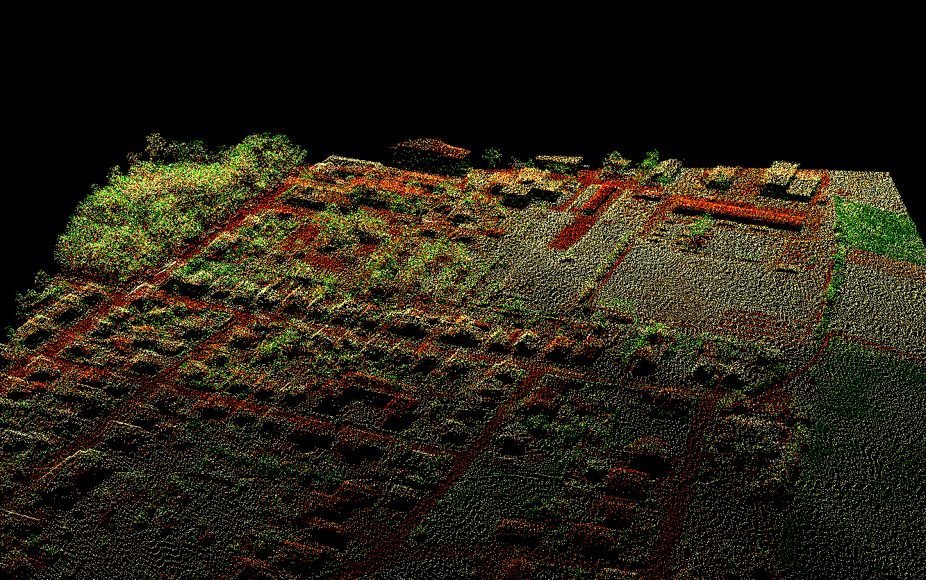
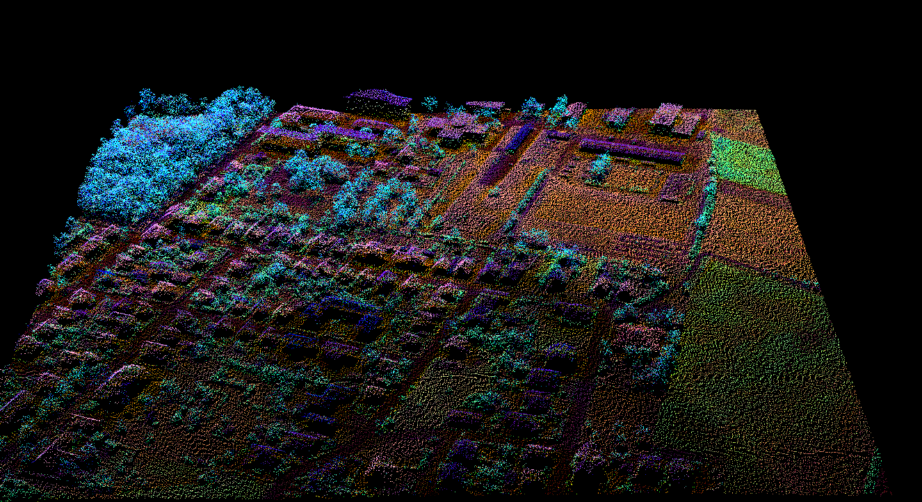
Finally, OpalsColorize allows comparison of three different attributes simultaneously, rescaling their values to the red, green and blue colour channels of the output respectively. The most popular combination of three attributes for full-waveform LIDAR is Reflectance --> Red, EchoWidth --> Green and NormalizedZ --> Blue, as this gives an intuitive output with green vegetation, red terrain and blue high points. If 3 attributes are specified in OpalsColorize, they are colored according to their order Red, Green, and Blue. Histogram equalization is essential, since the three variables have very different value ranges. Please note that no palette is specified: the colour scheme is produced by the mixing of the RGB channels. Three legend files are produced, one for each attribute
The output dataset can be used for understanding the connections between the different attributes and as a basis for selecting attributes for point cloud classification.
A. Zlinszky, A. Schroiff, J. Otepka, G. Mandlburger, N. Pfeifer "Simultaneous colour visualizations of multiple ALS point cloud attributes for land cover and vegetation analysis"; European Geosciences Union, General Assembly 2014 (EGU 2014), Wien. Full paper
 1.8.17