Technische Universität Wien
Orientation and Processing of Airborne Laser Scanning data
Department of Geodesy and Geoinformation - Research Groups Photogrammetry and Remote Sensing
Calculates a high quality Digital Terrain Model in hybrid grid structure (i.e. regular grid + structure lines).
Airborne Laser Scanning (ALS) provides a dense set of points located at arbitrary positions. The point densities are typically in the range of 1-20 points per square meter. ALS is also capable of penetrating vegetation through small gaps in the foliage and, thus, can provide the ground beneeth the canopy. One of the main applications of ALS is therefore the derivation of Digital Terrain Models (DTM). Interpolating the terrain surface is, however, the final step in a complex processing chain starting with waveform analysis, 3D point cloud derivation (Package opalsPreprocess), quality assessment (Package opalsQuality), geometric and radiometric calibration (Package opalsGeoref), derivation of 3D structure lines (Package opalsGeomorph), and filtering ground and off-terrain points (Package opalsClassify). In general, geo-statistical interpolation strategies have proven to deliver the best results. Kriging or linear prediction, respectively, are so-called BLUE (best linear unbiased estimators), but they are computationally expensive. Dense ALS point clouds therefore justify the usage of simpler interpolation techniques like moving least squares. Module DTM, in particular, uses linear or quadratic functional models (i.e. tilted planes or paraboloids). For each grid point the neigbouring laser points are used to locally fit such basic models and the grid height is calculated from the resulting geometry primitive. In addition to the point cloud, explicit line information e.g. from semi-automatic 3D structure line modelling (cf. Package opalsGeomorph) is considered within the DTM interpolation. Please note, that whereas the final goal of Module DTM is the construction of a hybrid DTM structure consisting of a regular elevation grid (i.e. height field) and vectors (interlinked structure lines), up to now the line information is specifically used for the grid point interpolation whereas the DTM is stored as a regular raster and a separate line structure file is written.
A single or multiple OPALS Datamanger (ODM) files containing, both, point and line data constitute the main input for Module DTM (inFile). The DTM raster (outFile) is stored in a GDAL (GeoData Abstraction Library) supported format. The grid spacing (gridSize) should be chosen to match the laser point density. As a rule of thumb, approximately 1-4 laser points should be used for the height estimation of a single grid point. Specification of the size of the internal processing and storage units (tileSize) is optional. Whereas larger tile sizes improve the computation performance they also require more RAM storage resources.
The neighbourhood definition is crucial for local surface fitting. Module DTM uses a generation based point selection strategy illustrated in Figure 1.
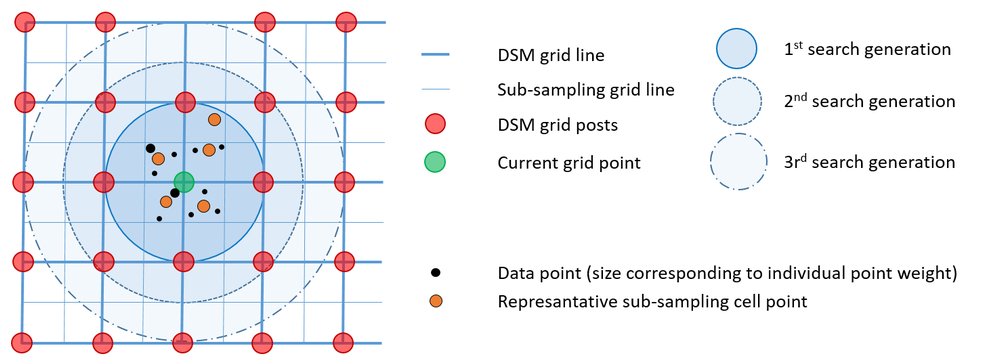
Data selection works as follows: The output grid structure is sub-sampled so that each output DTM grid cell is divided into four sub-sampling cells. The data points are then sorted into these sub-sampling cells. If more than one points falls within such a cell, a representative point is calculated based on weighted centre-of-gravity calculation. Therefore a user defined weight function can be specified (weightFunc). As a practical example for this, the user might want to favor points with a higher (raw) amplitude or (calibrated) reflectance over points with low signal strength. In this case the respective point attributes (amplitude, reflectance, intensity, etc.) can directly used as weight function but, however, arbitrarily complex weight functions can be specified in generic filter syntax. Once all the points are sorted into the respective subsampling cell, the generation based point selection starts with a search radius equal to the DTM grid size. In the 1st> generation all sub-sampling grid cells with a maximum distance to the investigated grid post of 1 * DTM grid width are considered. If the number of neighbouring points is less then the requested knn-count (neighbours) the search radius is extended by one sub-sampling grid cell (i.e. half of the DTM grid spacing) and all points of the circular ring are added. The procedure is repeated until either the knn point count is greater than or equal (neighbours) or the maximum search radius (searchRadius) is reached. Please note that, although this is a raster based point selection approach, still the arbitrary positions of the representative cell points are maintained. In addition to the point data, all line data in the vicinity of the grid point are considered within the interpolation.
Whereas moving least squares imply noise reduction and gross error filtering (at least to a certain degree), triangulations use the original unfiltered data for describing the interpolation surface. Hence, such surfaces contain measurement noise, gross errors and reflect the often random distribution of the input data. Therefore, grid models derived by moving least squares typically outperform tin based interpolators by precision and visual appearance. Nevertheless, tin based interpolators are well known and can easily support structure line information which is why Module DTM provides a Constraint Delaunay Triangulation (CDT) interpolator based on the CGAL library. For completeness, it is mentioned that the data selection parameters like neighbours, weightFunc, etc. do not influence the triangulated surface and therefore, they will be ignored during processing.
Based on the multi-threaded tile-wise processing strategy Module DTM provides two different triangulation strategies which will vary in processing speed and memory consumption:
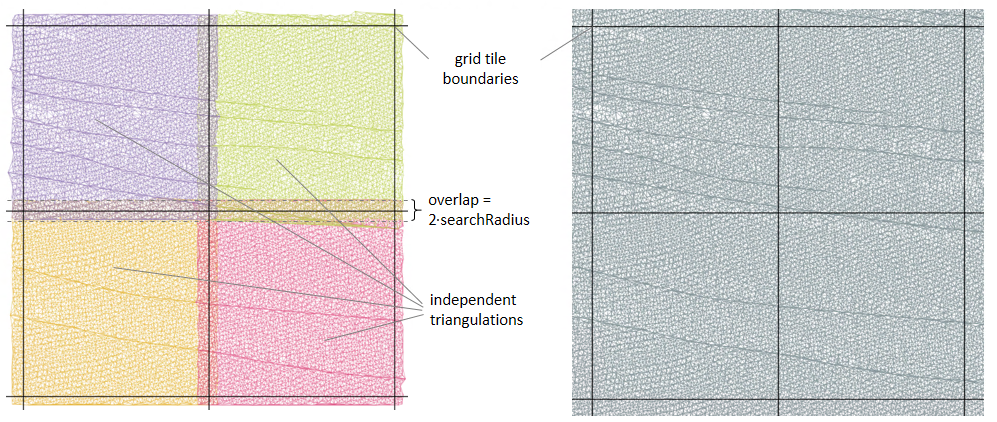
The tile-based triangulation strategy is activated by a searchRadius larger than zero which implicitly serves as overlap parameter (cf. Figure 2). Tile-based triangulation is typically faster and requires less memory since each processing thread has its own small triangulation object. This strategy, however, can result in interpolation artefacts due to differently formed triangles at the grid tile boundaries. Furthermore, large data gaps can lead to empty grid cell as visible in example 2. By increasing the searchRadius parameter which will lead to a large overlap, those issues can be eliminated or at least greatly reduced. Nevertheless, especially for data with inhomogeneous data distribution, interpolation artefacts may always occur. For such data sets the global triangulation strategy resolves those issues. There, one global triangulation object is created single-threaded which is then used by all interpolation threads. The downside of global triangulation strategy is that it requires enough memory to build a triangulation that contains all input data. So for huge data set it might be impossible to use the global triangulation strategy.
All remaining parameters are optional. As mentioned above, the primary aim of Module DTM is the derivation of a terrain model. Furthermore, additional feature models (feature) can be derived as by-products of the grid interpolation (i.e. without loss of performance). The following additional features are supported:
By default, the entire ODM content is used as input. Specific point/line data selection is enabled by providing an appropriate filter string (filter). In addition, a user defined limit can be specified (limit). By default, the height raster and the additional feature rasters are written to separate files. To generate a single multi-band raster file set multiBand=1. Please note, that all raster files are created in GeoTiff file format and the individual rasters are kept together by a GDAL Virtual Raster master file. Future releases will extend this concept to implement a hybrid DTM structure (i.e. joint storage of both raster and vector contents).
Possible values:
  delaunayTriangulation ... Delaunay triangulation interpolation
  movingPlanes ............ moving (tilted) plane interpolation
  kriging ................. kriging interpolation
Supported interpolation methods: movingPlanes|kriging.
Possible values:
  sigmaz ......... sigma z of grid post adjustment (i.e. std.dev. of the interpolated height)
  sigma0 ......... sigma 0 of grid post adjustment (i.e. std.dev. of the unit weight observation)
  pdens .......... point density estimate
  pcount ......... number of points used for interpolation of grid point
  excentricity ... distance between grid points - c.o.g. of data points
  slope .......... steepest slope [%] (deprecated: use slpPerc instead)
  slpPerc ........ steepest slope [%]
  slpDeg ......... steepest slope [deg]
  slpRad ......... steepest slope [rad]
  exposition ..... slope aspect [rad] (deprecated: use expoRad instead)
  exposRad ....... slope aspect [rad] (azimuth of steepest slope)
  exposDeg ....... slope aspect [deg] (azimuth of steepest slope)
  normalx ........ x-component of surface normal unit vector
  normaly ........ y-component of surface normal unit vector
If one or more features are specified, additional grid models in the same format and structure as the basic terrain model are derived. By default, a multiband raster is created in this case. Please note, that if each feature is written to a separate file (i.e. multiband=false) and if more than one output file is specified, the number of output file names must match the number of specified features: nr. outFile = nr. feat. + 1
The data used in the following examples are located in the $OPALS_ROOT/demo/ directory. As pre-processing step, the 3D point cloud (flyover.laz) and the 3D break lines (flyover_breaklines.shp) are imported into a single ODM file using the following command:
To create a 25cm DTM grid based using 12 nearest neighbours in a maximum search distance of 1.25m and additional feature models (surface normal vector and grid height precision) use the following command:
Visualizations of the resulting raster files (DTM shaded relief map, color coded sigmaZ, normalx and normaly map) are plotted in Figure 3:
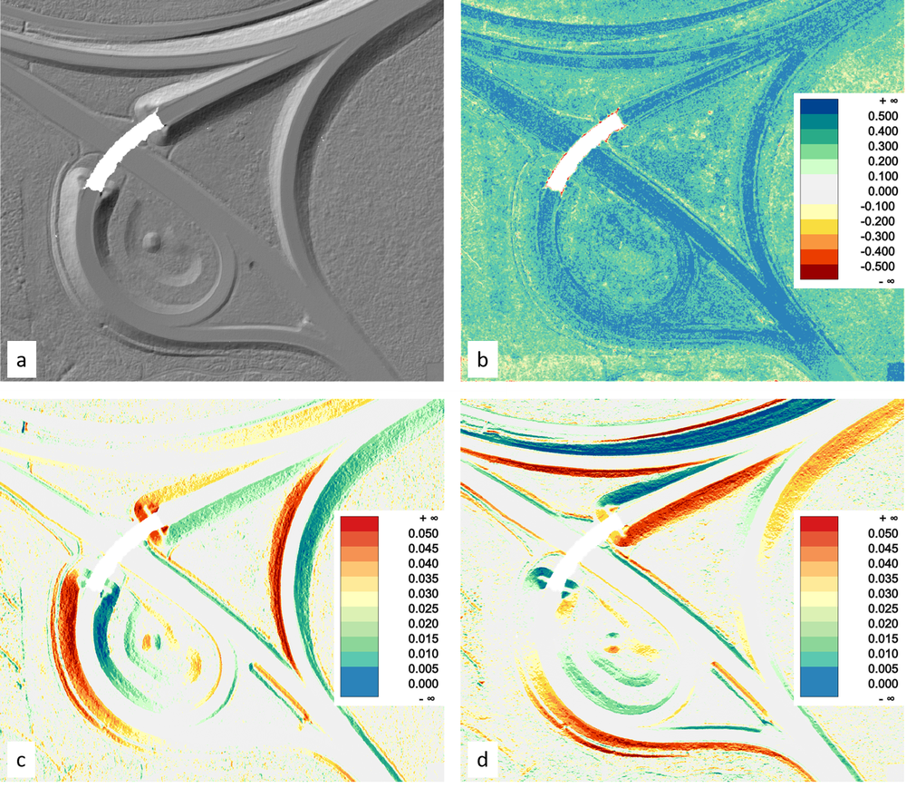
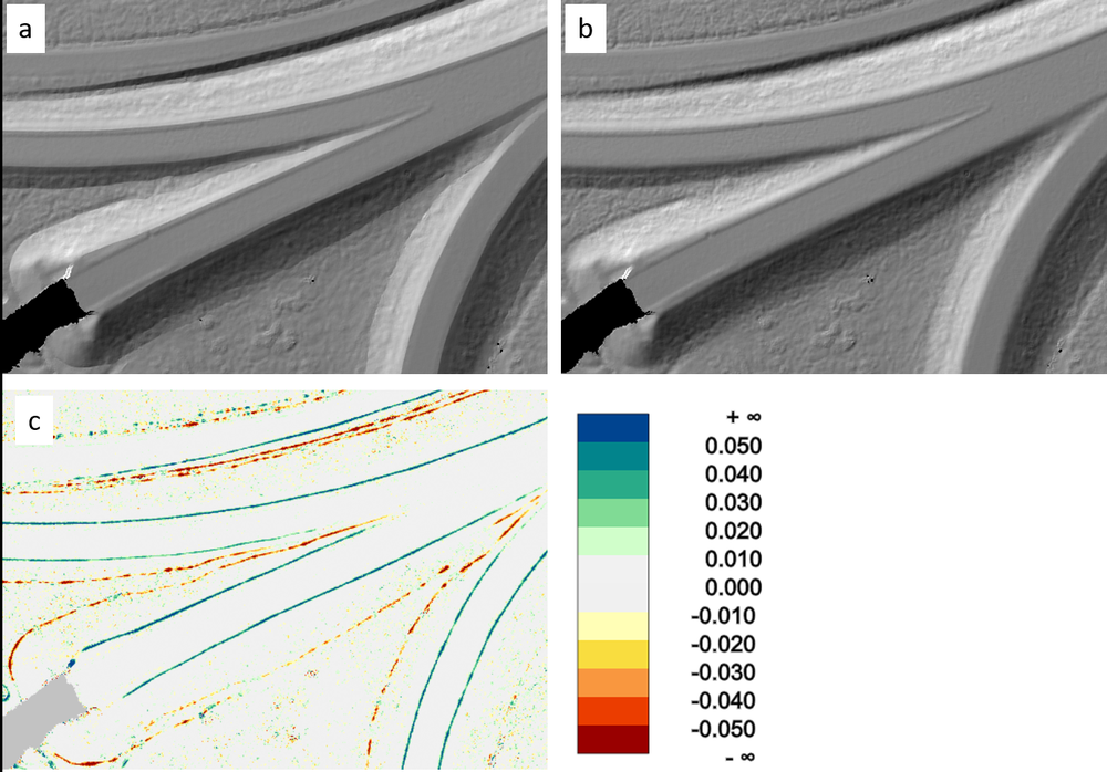
Figure 4 shows a detail of the shaded DTM relief compared to a variant without considering the breaklines in the surface interpolation (Module Grid):
In this example the triangulation interpolator is used and the effect of the two different triangulation strategies is shown. First, tile-based triangulation strategy using a 2m overlap (searchRadius -> 1) is applied and second, the global triangulation approach is used (searchRadius -> 0)
Figure 5 shows shaded reliefs of the two different triangulation strategies. As it can be seen the two final DTM model only differ at larger data gaps (cf. Figure 4a). For completeness it is mentioned that gaps in raster models can be specifically closed by applying Module FillGaps.
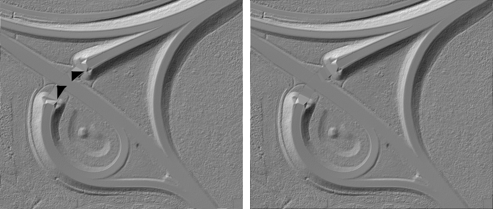
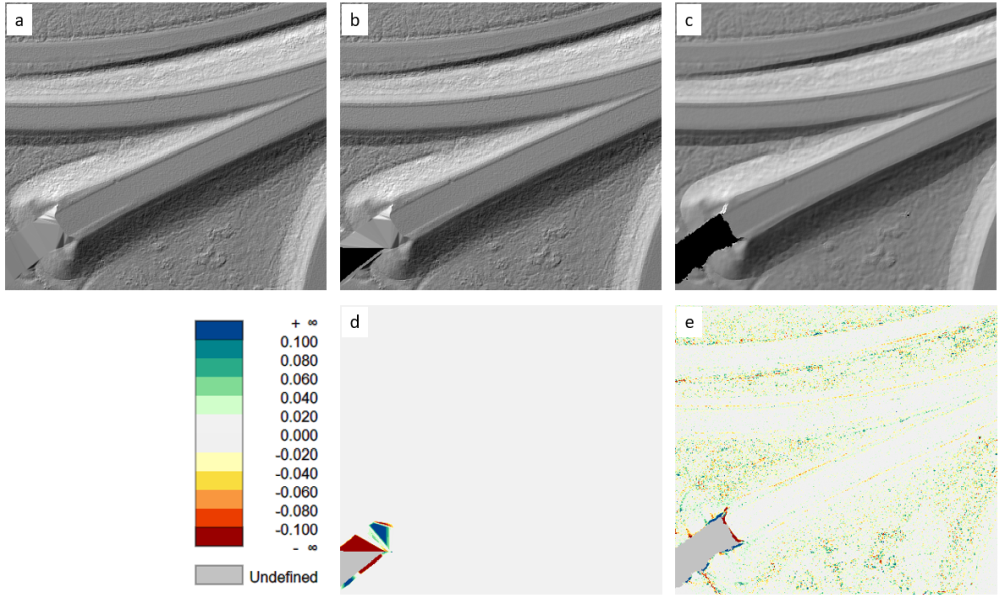
Figure 6 visualizes the differences of the different interpolators and triangulation strategies in a side-by-side figure. Whereas the two triangulation strategies only differ at data gaps (Figure 6d), the height differences between triangulation and moving plane interpolator show speckle patterns (Figure 6e) especially on vegetated and non-sealed ground. Those speckle range from 2 to 4 cm and result from a higher filtering/smoothing effect of the moving plane interpolator. When closely comparing the corresponding shaded relief (Figure 6b and 6c) this smoothing effect is directly visible.
 1.8.17