Technische Universität Wien
Orientation and Processing of Airborne Laser Scanning data
Department of Geodesy and Geoinformation - Research Groups Photogrammetry and Remote Sensing
Transforms points from scanner coordinates into geo-referenced coordinates by applying the sensor model (flight trajectory, mounting parameters).
For direct georeferencing of ALS data, the following input is required:
As output, we obtain the ALS ground points with respect to the defined spatial reference system (e.g. UTM33 North or geocentric WGS84), commonly termed as "world system".
We suppose that we have a strapdown inertial navigation system (INS), i.e. the inertial platform is fixed with respect to the aircraft's body. Consequently, its measurements are given in a body(-fixed) system \(B\). Its axes are defined as follows: \(x^B\): forward, \(y^B\): right, \(z^B\): down. Furthermore, we suppose that its origin corresponds to the current (interpolated) position of the flight trajectory.
Since the laser scanner data are usually not directly given in the body system \(B\), the so-called mounting calibration is required, which contains the transformation chain required to describe the transition from the scanner's coordinate system \(S\) to the body system \(B\). Figure 1 shows these two coordinate systems and two other intermediate systems \(S_0\) and \(M\).
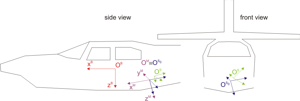
\(S_0\) is the scanner's coordinate system in zero position in case if a scanner tilting device is used (if not, the systems \(S_0\) and \(S\) are identical). In general, the system \(S\) is rotated (tilt rotation) and shifted (tilt shift) with respect to the system \(S_0\).
The mounting system \(M\) is defined as follows: Its axes result from cyclic permutation (scanner system) of those of system \(S_0\) in such a way that they are approximately parallel to those of the body system \(B\). The systems \(M\) and \(S_0\) have the same origin. The mount system is (usually slightly) rotated (mounting rotation) and shifted (mounting shift) with respect to the body system.
Using matrix notation, the relations between these coordinate systems may be described as follows:
\(\mathbf{x}^B=\mathbf{R}_M^B\cdot\mathbf{x}^M + t_M^B\)
\( \mathbf{x}^{M}=\mathbf{R}_{S_0}^M\cdot\mathbf{x}^{S_0}\)
\( \mathbf{x}^{S_0}=\mathbf{R}_S^{S_0}\cdot\mathbf{x}^S + t_S^{S_0} \)
The direct relation between the systems \(S_0\) and \(B\) is:
\( \mathbf{x}^B=\mathbf{R}_M^B\cdot\mathbf{R}_{S_0}^M\cdot\mathbf{x}^{S_0}+t_M^B=\mathbf{R}_{S_0}^B\cdot\mathbf{x}^{S_0}+t_{S_0}^B \)
General notes on notation:
Apart from the above-mentioned geometric transformation elements, the mounting calibration contains the time offset \(\Delta t\) (time lag) of the trajectory time system with respect to the laserscanner time system, too.
The parameters of the mounting calibration may be specified using a string according to the following EBNF (Extended Backus-Naur Form) syntax:
The following mounting parameters may be specified:
time lag: This is the time offset \(\Delta t\) of the trajectory time system with respect to the laser scanner system (i.e., this value has to be subtracted from a trajectory time stamp in order to obtain the same point of time in the scanner's time system)
scanner system: A sequence of 3 directions out of the set {F(ront),B(ack),L(eft),R(ight),U(p),D(own)} is used to specify the approximate attitude of the zero-tilted scanner system \(S_0\) - note: NOT that of the scanner system \(S\) (!) - with respect to the body system \(B\) (see figure 1). The direction sequence is restricted to the 24 possible right-handed systems. Based on this input, the rotation matrix \(\mathbf{R}_{S_0}^M\) (mentioned in the previous section) is determined. For example, in case of figure 1, the 3 axes of system \(S_0\) point down, back, and left (here, it is not specified which of the axes is X,Y,Z). Since we support only right-handed systems, the set-up of this example corresponds to one of the 3 possible sequences "D-B-L", "B-L-D", "L-D-B".
For example, "SCANNERSYS(D-B-L)" yields \( \mathbf{R}_{S_0}^M = \begin{pmatrix} 0 & -1 & 0 \\ 0 & 0 & -1 \\ 1 & 0 & 0 \end{pmatrix} \).
mounting rotation: The rotation from the system \(M\) into the system \(B\)
mounting shift: The translation (shift) from the system \(S_0\) into the system \(B\)
tilt rotation: The rotation from the system \(S\) into the system \(S_0\)
tilt shift: The translation (shift) from the system \(S\) into the system \(S_0\)
Hence, from the point of view of these transformation elements, the above-mentioned systems take role as a global or a local system.
The next section describes how to specify a rotation and/or a shift using the provided syntax.
Using the above-introduced matrix notation, a congruent (6-parameter) transformation from a local system \(L\) into a global system \(G\) may be described as:
\( \mathbf{x}^G=\mathbf{R}_L^G\cdot\mathbf{x}^L + t_L^G \Longleftrightarrow \mathbf{x}^L={(\mathbf{R}_L^G)}^T\cdot(\mathbf{x}^G-t_L^G) \)
In the same way, the inverse transformation may be described as:
\( \mathbf{x}^L=\mathbf{R}_G^L\cdot\mathbf{x}^G + t_G^L \Longleftrightarrow \mathbf{x}^G={(\mathbf{R}_G^L)}^T\cdot(\mathbf{x}^L-t_G^L) \)
Consequently, the following relations hold:
\( \mathbf{R}_L^G={(\mathbf{R}_G^L)}^T \) and \( t_L^G=-\mathbf{R}_L^G\cdot t_G^L \)
The above-decribed syntax allows the user to specify a rotation and/or a shift in different ways:
Specifying a shift:
Depending on the refsys parameter, a shift vector may be specified either as \(t_L^G\) ("GLOBAL": the shift vector corresponds to the position of the local system's origin expressed in the global system) or as \(t_G^L\) ("LOCAL": the shift vector corresponds to the position of the global system's origin expressed in the local system).
Note: Since the system \(M\) is just an auxiliary system with hardly practical relevance, the mounting shift expressed in the local system is NOT \(t_B^M\) BUT \(t_B^{S_0}\) (!). Hence, the mounting shift expressed in the global system \(B\) may be determined by \( t_{S_0}^B=t_M^B=-\mathbf{R}_{S_0}^B\cdot t_B^{S_0}=-\mathbf{R}_M^B\cdot\mathbf{R}_{S_0}^M\cdot t_B^{S_0} \)
Specifying a rotation:
Basically, there are three possibilities to specify a rotation:
Specifying a rotation by 3 angles:
Note: when specifying a rotation by 3 angles \(\alpha\), \(\beta\), \(\gamma\), the resulting matrix will be anyway (!) \(\mathbf{R}_L^G\) (i.e. rotation from the local into the global system). The refsys parameter specifies which system the angles are related to (i.e. around the axes of which system the rotations are performed). Depending on the refsys parameter, the entire rotation matrix is created either by right or by left multiplication of the sub-matrices \(\mathbf{R}_1(\alpha)\), \(\mathbf{R}_2(\beta)\), \(\mathbf{R}_3(\gamma)\):
"GLOBAL": \( \mathbf{R}_L^G=\mathbf{R}_1(\alpha)\cdot\mathbf{R}_2(\beta)\cdot\mathbf{R}_3(\gamma) \)
"LOCAL": \( \mathbf{R}_L^G=\mathbf{R}_3(\gamma)\cdot\mathbf{R}_2(\beta)\cdot\mathbf{R}_1(\alpha) \)
Depending on the parameter axis hierarchy, the submatrices \(\mathbf{R}_k(\varphi_k)\) are replaced by \(\mathbf{R}_x(\varphi_x)\), \(\mathbf{R}_y(\varphi_y)\), \(\mathbf{R}_z(\varphi_z)\), where
\( \mathbf{R}_x(\varphi)=\begin{pmatrix}1 & 0 & 0 \\ 0 & \cos\varphi_x & -\sin\varphi_x \\ 0 & \sin\varphi_x & \cos\varphi_x \end{pmatrix} \) and \( \mathbf{R}_y(\varphi)=\begin{pmatrix}\cos\varphi_y & 0 & \sin\varphi_y \\ 0 & 1 & 0 \\ -\sin\varphi_y & 0 & \cos\varphi_y \end{pmatrix} \) and \( \mathbf{R}_z(\varphi)=\begin{pmatrix}\cos\varphi_z & -\sin\varphi_z & 0 \\ \sin\varphi_z & \cos\varphi_z & 0 \\ 0 & 0 & 1 \end{pmatrix} \).
The default rotation sense of the angles \(\alpha\), \(\beta\), \(\gamma\) is counter-clockwise ("CCW") (mathematically positive when looking against the respective rotation axis). It may be as well specified as clockwise ("CW") using the parameter rotation sense: in this case, all the 3 angles are multiplied by (-1) before being evaluated in the submatrices.
The parameter units allows the user to select the angle units, where "DEG", "GRAD", or "RAD" may be specified (the default is "DEG").
For example, the specification of the mounting rotation matrix by three angles \(\alpha\) (roll), \(\beta\) (pitch), \(\gamma\) (yaw) according to the aviation ARINC 705 (see section Alignment of the aircraft) corresponds to refsys="=LOCAL", axis hierarchy="AXISHIERARCHY(X-Y-Z)" and rotation sense="SENSEOFROT(CCW)". \( \Longrightarrow \mathbf{R}_L^G=\mathbf{R}_z(\gamma)\cdot\mathbf{R}_y(\beta)\cdot\mathbf{R}_x(\alpha) \)
For the following examples, we define \( \rho=\frac{180}{\pi} \).
Example 1:
User input:
This is equivalent to the complete input:
It yields:
\(\Delta t=0.0\), \( \mathbf{R}_{S_0}^M = \begin{pmatrix} 0 & 1 & 0 \\ 0 & 0 & 1 \\ 1 & 0 & 0 \end{pmatrix} \), \( \mathbf{R}_M^B = \mathbf{R}_z(\frac{-0.37684}{\rho})\cdot\mathbf{R}_y(\frac{0.2479}{\rho})\cdot\mathbf{R}_x(\frac{0.07346}{\rho})= \begin{pmatrix} 0.9999690 & 0.0065826 & 0.0043181 \\ -0.0065770 & 0.9999775 & -0.0013105 \\ -0.0043267 & 0.0012821 & 0.9999898 \end{pmatrix} \), \( \mathbf{t}_M^B = \mathbf{t}_{S_0}^B = \begin{pmatrix}-0.7834 \\ 0.193422 \\ 0.07165\end{pmatrix} \), \( \mathbf{R}_S^{S_0} = \mathbf{I} \), \( \mathbf{t}_S^{S_0} = \mathbf{o} \)
Example 2:
User input:
This is equivalent to the complete input:
It yields:
\(\Delta t=-0.007\), \( \mathbf{R}_{S_0}^M = \begin{pmatrix} 0 & 1 & 0 \\ 1 & 0 & 0 \\ 0 & 0 & -1 \end{pmatrix} \), \( \mathbf{R}_M^B = \mathbf{R}_y(\frac{0.07346}{\rho})\cdot\mathbf{R}_x(\frac{0.2479}{\rho})\cdot\mathbf{R}_z(\frac{-0.37684}{\rho})= \begin{pmatrix} 0.9999775 & 0.0065826 & 0.0012821 \\ -0.0065770 & 0.9999690 & -0.0043267 \\ -0.0013105 & 0.0043181 & 0.9999898 \end{pmatrix} \), \( \mathbf{t}_M^B = \mathbf{t}_{S_0}^B = \begin{pmatrix}-0.927 \\ 0.014 \\ 0.053\end{pmatrix} \),
\( \mathbf{R}_S^{S_0} = \begin{pmatrix} 0.4472136 & 0.0000000 & -0.8944272 \\ 0.0000000 & 1.0000000 & 0.0000000 \\ 0.8944272 & 0.0000000 & 0.4472136 \end{pmatrix} \), \( \mathbf{t}_{S_0}^S = \begin{pmatrix} 0.1204 \\ 0.0564 \\ -0.0134 \end{pmatrix} \Longrightarrow \mathbf{t}_S^{S_0} = -\mathbf{R}_S^{S_0}\cdot\mathbf{t}_{S_0}^S = \begin{pmatrix}-0.0658 \\ -0.0564 \\ -0.1017 \end{pmatrix} \)
Example 3:
User input:
This is equivalent to the complete input:
It yields the same mounting calibration as example 1:
\(\Delta t=0.0\), \( \mathbf{R}_{S_0}^M = \begin{pmatrix} 0 & 1 & 0 \\ 0 & 0 & 1 \\ 1 & 0 & 0 \end{pmatrix} \), \( \mathbf{R}_M^B =\begin{pmatrix} 0.9999690 & 0.0065826 & 0.0043181 \\ -0.0065770 & 0.9999775 & -0.0013105 \\ -0.0043267 & 0.0012821 & 0.9999898 \end{pmatrix} \), \( \mathbf{t}_B^{S_0}= \begin{pmatrix} -0.068013 \\ 0.784958 \\ -0.188353 \end{pmatrix} \Longrightarrow \mathbf{t}_M^B =\mathbf{t}_{S_0}^B =-\mathbf{R}_M^B\cdot\mathbf{R}_{S_0}^M\cdot\mathbf{t}_B^{S_0}=\begin{pmatrix}-0.7834 \\ 0.193422 \\ 0.07165\end{pmatrix} \),
\( \mathbf{R}_S^{S_0} = \mathbf{I} \), \( \mathbf{t}_S^{S_0} = \mathbf{o} \)
Example 4:
User input:
This is equivalent to the complete input:
It yields:
\(\Delta t=0.0\), \( \mathbf{R}_{S_0}^M = \begin{pmatrix} 0 & -1 & 0 \\ 0 & 0 & -1 \\ 1 & 0 & 0 \end{pmatrix} \), \( \mathbf{R}_B^M =\begin{pmatrix} 0.9999690 & 0.0065826 & 0.0043181 \\ -0.0065770 & 0.9999775 & -0.0013105 \\ -0.0043267 & 0.0012821 & 0.9999898 \end{pmatrix}\) \( \Longrightarrow \mathbf{R}_M^B={(\mathbf{R}_B^M)}^T=\begin{pmatrix} 0.9999690 & -0.0065770 & -0.0043267 \\ 0.0065826 & 0.9999775 & 0.0012821 \\ 0.0043181 & -0.0013105 & 0.9999898 \end{pmatrix} \),
\( \mathbf{t}_B^{S_0}= \begin{pmatrix} -0.068013 \\ 0.784958 \\ -0.188353 \end{pmatrix} \Longrightarrow \mathbf{t}_M^B =\mathbf{t}_{S_0}^B =-\mathbf{R}_M^B\cdot\mathbf{R}_{S_0}^M\cdot\mathbf{t}_B^{S_0}=\begin{pmatrix}-0.7859 \\ -0.183094 \\ 0.07165\end{pmatrix} \),
\( \mathbf{R}_{S_0}^S = \begin{pmatrix} 0.9805807 & 0.0000000 & -0.1961161 \\ 0.0000000 & 1.0000000 & 0.0000000 \\ 0.1961161 & 0.0000000 & 0.4472136 \end{pmatrix} \Longrightarrow \mathbf{R}_S^{S_0} = {(\mathbf{R}_{S_0}^S)}^T = \begin{pmatrix} 0.9805807 & 0.0000000 & 0.1961161 \\ 0.0000000 & 1.0000000 & 0.0000000 \\ -0.1961161 & 0.0000000 & 0.4472136 \end{pmatrix}\), \( \mathbf{t}_S^{S_0} = \mathbf{o} \)
According to the aviation norm ARINC 705 (Bäumker and Heimes, 2001), we use the following definitions (Figure 2):
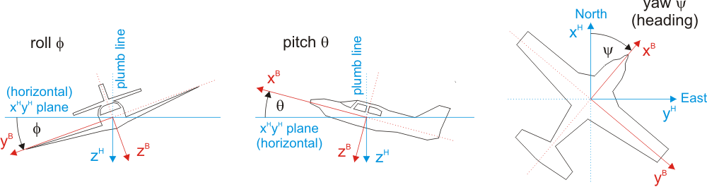
The entire rotation matrix \(\mathbf{R}_B^H\) transforms a point from the body system \(B\) into the system of the local horizon \(H\):
\(\mathbf{x}^H=\mathbf{R}_B^H\cdot\mathbf{x}^B\)
where
\(\mathbf{x}^B={\begin{pmatrix}x^B & y^B & z^B \end{pmatrix}}^T\), \(\mathbf{x}^H={\begin{pmatrix}x^H & y^H & z^H \end{pmatrix}}^T\)
and
\(\mathbf{R}_B^H=\mathbf{R}_z(\psi)\cdot\mathbf{R}_y(\theta)\cdot\mathbf{R}_x(\phi)=\)
\(=\begin{pmatrix}\cos\psi & -\sin\psi & 0 \\ \sin\psi & \cos\psi & 0 \\ 0 & 0 & 1 \end{pmatrix}\cdot \begin{pmatrix}\cos\theta & 0 & \sin\theta \\ 0 & 1 & 0 \\ -\sin\theta & 0 & \cos\theta \end{pmatrix}\cdot \begin{pmatrix}1 & 0 & 0 \\ 0 & \cos\phi & -\sin\phi \\ 0 & \sin\phi & \cos\phi \end{pmatrix}=\) \(\begin{pmatrix}\cos\psi\cdot\cos\theta & \cos\psi\cdot\sin\theta\cdot\sin\phi-\sin\psi\cdot\cos\phi & \cos\psi\cdot\sin\theta\cdot\cos\phi+\sin\psi\cdot\sin\phi \\ \sin\psi\cdot\cos\theta & \sin\psi\cdot\sin\theta\cdot\sin\phi+\cos\psi\cdot\cos\phi & \sin\psi\cdot\sin\theta\cdot\cos\phi-\cos\psi\cdot\sin\phi \\ -\sin\theta & \cos\theta\cdot\sin\phi & \cos\theta\cdot\cos\phi \end{pmatrix}\)
Note: In compliance with the notation of the previous section, the columns of the rotation matrix \(\mathbf{R}_B^H\) correspond to the unit vectors of the axes of system B expressed in system H.
Note: If a map projection is used as global coordinate system (see next section), the yaw angle \(\psi\) will be automatically corrected for the meridian convergence. In this case, the system \(H\) is not oriented towards True North but towards Grid North.
The world coordinate system may be specified by the global parameter coord_ref_sys.
Basically, two types of world coordinate systems are supported by this module:
Note: Geographic coordinates (latitude, longitude, ellipsoidal height) have to be converted into one of the above-mentioned system types first.
The specification of the world coordinate system should contain the parameters \(a\) (semi major axis) and \(f\) (flattening) of the reference ellipsoid (if not, the parameters of the WGS84 ellipsoid are used instead). In case of a transverse mercator projection, the parameters false_easting (default: 0.0), false_northing (default: 0.0), and scale_factor (default: 1.0) should be contained, too.
For example, the system "UTM zone 33 - northern hemisphere" may be specified either by the WKT string
or by its EPSG code
In case of a geocentric system, a ground point given in the local horizon system \(H\) is transformed into the world system \(W\) by:
\(\mathbf{x}^W=\mathbf{R}_H^W\cdot\mathbf{x}^H+\mathbf{t}_H^W\)
where \(\mathbf{R}_H^W\) is a rotation matrix, which describes the attitude of the local horizon system \(H\) with respect to the world system \(W\), and where \(\mathbf{t}_H^W=\mathbf{t}_B^W\) is the current (interpolated) trajectory point given in the world system \(W\).
In case of a Transverse Mercator map projection, beside the meridian convergence (already considered by correction of the yaw angle), the projection's length distortion and earth curvature are taken into account to transform a ground point into the "projected" horizon system \(H_P\) (having the same origin as \(H\)), from where it is finally translated into the world system \(W\):
\( \mathbf{x}^W = \mathbf{x}^{H_P}+\mathbf{t}_H^W = F(\mathbf{x}^H, \mathbf{t}_H^W, a, f)+\mathbf{t}_H^W \)
where \( F(\mathbf{x}^H, \mathbf{t}_H^W, a, f) \) contains the correction terms necessary due to the (space-dependent) length distortion and earth curvature
At least one trajectory file is required for this module.
A trajectory file must contain a set of at least 2 records containing the following data:
The module tries to recognise the trajectory format based on its content if not specified. The standard input format is the "trajectory file format (trj)" which supports ASCII and binary mode. The 7 columns can be given in two different orders:
Since the gps time is excepted to be in ascending order, the two formats can be easily differentiated without any specification. In cases where both tested columns are in ascending order stdDevMAD (robust standard deviation estimator computed from the median of absolute deviations from the median) is used as decision criterion. The columns with the lower stdDevMAD is assumed to be the gps time column (In rare cases where the heuristic doesn't recognise the file format correctly, one can always provide an format definition as described below). Whereas all angles columns are stored in radiant within the ODM (see ODM as a database table), the trajectory format assumes the angle to be given in degrees. Hence, while reading the angles are automatically converted. Please note, that in binary mode the the first 4 values are read as doubles (8 bytes per values) and the 3 angles as floats (4 bytes per value).
In case your trajectory file doesn't match the format described above, it is possible to create an appropriate OPALS format description (see OPALS Generic Format) and specify those as tFormat parameter. Please note that angle values are expected in radians which can be simply realised specifying an appropriate transformation in the OPALS format description file.
If two ore more trajectory files are given, their time ranges (intervals between first and last entry) must not overlap. Furthermore, the time range of a scanner file must be completely within the time range of one trajectory.
The data used in the following examples are located in the demo directory.
We start from the given demo file 060622_173547.sdf. First, Module Fullwave has to be applied to this file in order to generate the file 060622_173547.sdc:
The associated trajectory file F002_20060622_UTM33_part.txt is given in UTM 33, the global parameter coord_ref_sys may be set as described in the example above.
In this example, we have a Down-Front-Right scanner system (without tilting). The time lag is -3.2 milliseconds.
As result, we obtain the LAS file 060622_173547_dirGeoref.las containing the georeferenced point cloud.
We are starting from the demo file stripPart.sdc. Since the trajectory file trjPart_geoc.txt is given in geocentric WGS 84 coordinates, we set the global parameter coord_ref_sys to
or to
In this example, we have a Down-Back-Left scanner system (without tilting). There is no time lag.
As result, we obtain the LAS file stripPart_dirGeoref.las containing the georeferenced point cloud.
Bäumker, M., F.-J. Heimes (2001): New Calibration and Computing Method for Direct Georeferencing of Image and Scanner Data Using the Position and Angular Data of an Hybrid Navigation System. In: Proceedings OEEPE-Workshop Integrated Sensor Orientation, Hannover, 17.-18. Sept. 2001.
 1.8.17