Technische Universität Wien
Orientation and Processing of Airborne Laser Scanning data
Department of Geodesy and Geoinformation - Research Groups Photogrammetry and Remote Sensing
Models 3D structure lines based on a point cloud (ODM) and 2D line approximations.
The 3D point cloud (inFile) in ODM file format and 2D approximations of the structure lines (approxFile, valid formats: ESRI shapefile, (Binary) Winput) constitute the main input for Module LineModeler. The resulting 3D structure/break lines are stored in a vector data file (outFile) either in ODM, ESRI shapefile, or (Binary) Winput file format (oFormat). By default, the entire 3D point cloud is used for structure line modeling. However, the input points can also be restricted using an appropriate filter string. For processing only a subset of lines a list of line ids or a single textfile containting the respective line ids can be specified (processId). Please note, that for line approximations provided in Winput file format, the is correspond to the structure number, whereas else (i.e. Shape and ODM) the consecutive line numbers are used. The same strategy can be applied to skip processing of certain lines via parameter ignoreId.
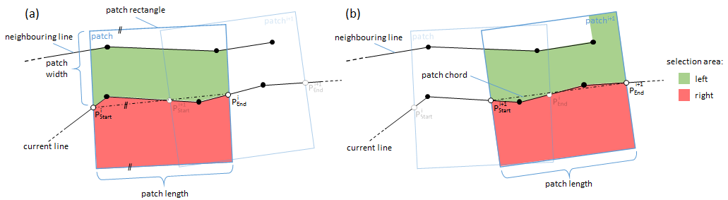
The general 3D modeling strategy of Module LineModeler is based on the intersection of local geometry primitives (plane, cone, or polynomial cylinder). The length and width of the surface elements to the left and the right of the 2D approximation can be set by the parameters patchLength and patchWidth. Please note, that a minimum and a maximum length can be specified denoting the smallest and largest longitudinal extension of the local surface elements. For the patch width either one value (symmetrical width to the left and the right of the 2D line approximation) or two values (1st=width left, 2nd=width right) are expected. Although usually a constant patch width is employed for modelling the entire line network, the maximum width is, however, locally constrained by the neighbouring 2D line approximations to ensure that a local surface element covers a smooth surface (see Figure 1). The patch length is automatically adjusted by Module LineModeler based on the curvature of the 2D approximations (i.e. the straighter the line progression, the longer the patch). In addition to the patch length and width, lower and upper bounds for the number of points within a single geometry primitive can be set (pointCount).
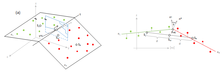
Once the points to the left and the right have been selected, local geometry primitive fitting is performed. It is important to know that both geometry primitives (left and right) are estimated in an integrated least-squares adjustment minimizing the vertical point-to-surface-patch deviations while considering the line approximations as additional observations. The latter helps to stabilize the results in awkward point configurations. Currently, three different patch pair fitting methods are implemented. The standard model is the plane pair fit as shown in Figure 2a. The actual result of each patch adjustment is a representative point P, the tangent t, the intersection angle, and several accuracy (σ) values. To avoid extrapolations the representative point P is computed by intersecting the two patch planes with a vertical plane that contains the center of gravity (COG) of the left (SL) and the right (SR) point set.
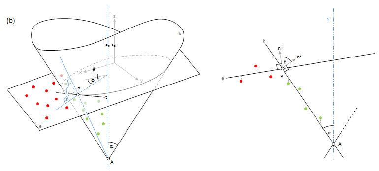
In case the 2D line approximation is strongly curved within the current patch, the modeling strategy computes a plane pair fit and a plane-cone fit. As can be seen in Figure 2b the used cone model is a circular cone with a vertical axis. The results of the plane-cone fit are selected if the σ0 a-posteriori is lower than the σ0 a-posteriori of plane pair fit. To compute the representative point P a vertical plane containing the COGs of both point sets is computed and intersected with the adjusted plane and cone. In general, there are two solutions for P which is why the distance to the approximation line is used to select the correct one.
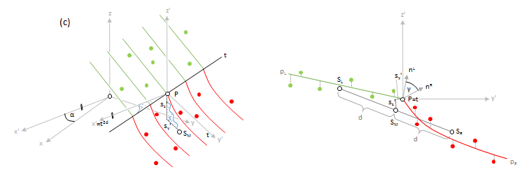
In cases were the surface is curved perpendicular to structure line but straight in line direction, plane and cone primitives sometimes deliver unsatisfactory results. For such situation a 2nd order polynomial cylinder model was developed as shown in Figure 2c. From a geometrical point of view, the model consists of two cylindrical surfaces that are formed by the motion of two parabolic curves (the generators) across the intersection line (the directrix). Testing the statistical significance of the quadratic terms helps reducing over parameterisation. The quadratic term is deactivated if not statitically significant, and the adjustment is repeated in this case. Hence, if both quadratic terms are deactivated, the model is identical to the standard plane pair model. In spite of the significance test, the model is less robust to imperfectly filtered ground points or irregular point arrangements. In case of doubt the plane pair fit is used as a fall back strategy. Currently, the polynomial pair fit is only used if:
Individual point weights are used within patch pair fitting procedure. Points located in the middle of the patch hereby get a higher weight compared to points at the patch border. This applies both to the longitudinal and transversial direction. In both cases, a gaussian curve is used with weights of 1 in the middle and approximately 0.5 at the border. In addition to that, the height precision of the 3D points and the planimetric precision of the line approximations can be specified via &sigma a-priori. Basically, two values are expected (1st value=height precision of 3D points, 2nd value=planimetric precision of 2D line approximations). If only one value is provided, the planimetric precision is set to 3 times the height precision. Whereas the above mentioned parameters provide user control of the geometry pair fitting, the distance between to patch centers along the line can be defined via parameter overlap. Again, two values denoting the upper and a lower bound for the potential patch overlap are accepted. Internally, the algorithm adapts the actual overlap depending on the local surface shape. A large overlap is used in high curvature areas (e.g. at U-turns at the end of ditch, etc.) and a small overlap is employed if the line progression is rather straight.
As stated before, the course of the 3D structure line is modeled by intersecting local geometry primetives wherever possible. However, the planimetric uncertainty increases with decreasing intersection angles. Therefore it is possible to specify a critical intersection angle (minAngle). If the patch pair intersection angle is smaller than the specified value, the elevation is derived from a one-sided plane and the planimitric position of the 2D line approximation is preserved. If plane fitting succeeds for both the left and the right plane, the more horizontal plane is used for the heigth estimation. In case the output is requested in ODM file format, all result parameters of the geometry fit are stored for each patch center point. Please note, that no matter which output format is chosen for the final 3D structure lines, the ODM containing the above mentioned metadata is stored in any case. The most important parameters are:
After modeling an entire line as a sequence of local patches of arbitrary length, a homogeneous point spacing along the 3D strucutre line is established by interpolating intermediate line vertices in approximately regular intervals (samplingDist). Cubic Bezier curves based on the 3D patch reference point positions and the corresponding 3D tangent directions of two adjacent patches are used for the line densification. Whereas generally all lines (cf. processId and ignoreId) above) are processed only those lines meeting a miminum user-defined length (minLength) are considered for output to suppresss overly short lines.
Once processing of a single line is completed, a quality assement is carried out. Quality indicators are provided as aggregated statistics for the entire line which might consist of severel (continuous) line parts (due to data voids in the 3D pint cloud, etc.). The quality level is described in school grade catagories (very good, good, moderate, sufficient, not sufficient). An additional class is provided for all lines which are topologically inconsistent (self intersections, etc.). The classification rule is as follows:
Unsufficient
Please note that, as mentioned before, more detailed metadata (on patch level) are available in the ODM output file.
The structure lines are provided in (i) ODM, and (iia) ESRI shapefile, or (iib)(Binary) Winput file format. In case of (Binary) Winput a separate output file is created for each catagory (very good, good, etc.). Furthermore, Winput does not provide the capability to store additional attributes. For ESRI shapefiles, a single file is created and the line id as well as the quality level (_origId, _quality) are provided as attributes in the corresponding database (dbf) file. Furthermore, a secondary output file containing the individual line segments is provided. For each segment the following attributes are available: (i) _id, (ii) _segmentId, (iii) _origId, and (iv) _curvature. Whereas _id constitutes a countinuous counter, _segmentId denotes the index of a segement within a certain line, _origId the id of the corresponding 3D structure line and, finally, _curvature a concave/convex indicator.
The data used in the following example can be found in the $OPALS_ROOT/demo/ directory. As a prerequisite the data of (flyover.laz) are imported into an OPALS data manager, and 2D line approximations are derived following the procedure detailed in the examples section of Module LineTopology.
The first example reads the paprameters from the configuration file (lineModeler.cfg) provided in the demo directory.
The 3d structure lines can then by derived simply by passing the path and name of the configuration file as well as the path names of the point cloud (inFile), of the 2d line approximations (approxFile) and of the resulting 3D structure lines (outFile).
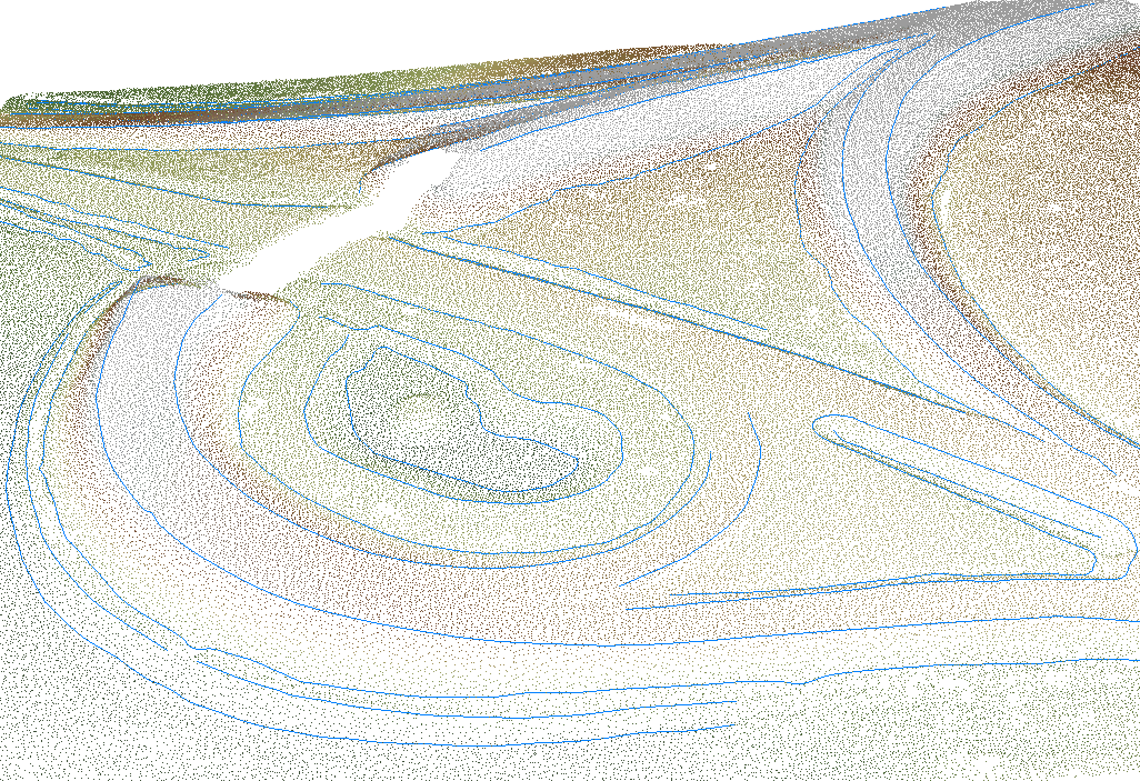
The resulting 3D structure lines are plotted in Figure 1 together with the original 3D point cloud.
A quality measure for the resulting lines is the distance to the DTM surface. It can be calculated for each node of the structure lines. First, the nodes have to be exported as (xyz)-Points, and then imported to an odm again:
Using opalsAddInfo, the distances to the DTM can be calculated:
With a custom format definition file (addons\formatdef\lineModelerShape.xml), the attribute can be exported to a shapefile for further investigation:
G. Mandlburger, J. Otepka, C. Briese, W. Mücke, G. Summer, N. Pfeifer, S. Baltrusch, C. Dorn, H. Brockmann: Automatische Ableitung von Strukturlinien aus 3D-Punktwolken. in: "Dreiländertagung der SGPF, DGPF und OVG: Lösungen für eine Welt im Wandel", T. Kersten (ed.); Publikationen der Deutschen Gesellschaft für Photogrammetrie, Fernerkundung und Geoinformation e.V., Band 25 (2016), ISSN: 0942-2870; 131 - 142.
Otepka, J., Mandlburger, G., Briese, C. und Pfeifer, N.: Fortschritte bei der automatischen Ableitung von Strukturlinien aus 3D-Punktwolken. 19. Internationale Geodätische Woche Obergurgl 2017, Hanke, K. & Weinold, Th. (Hrsg.) Herbert Wichmann Verlag, VDE VERLAG GMBH, Berlin/Offenbach. ISBN 978-3-87907-xxx
 1.8.17