Module ICP
See also
opals::IICP

Aim of module

Performs orientation (co-registration) of multiple point cloud datasets using the Iterative Closest Point algorithm.

Requirements for usage of opalsICP

This module requires the installation of the Matlab runtime.

General description

The Iterative Closest Point (ICP) algorithm (Chen & Medioni (1991), Besl & McKay (1992)) improves the alignment of two (or more) point clouds by minimizing iteratively the discrepancies within the overlap area of these point clouds. Nowadays the term ICP does not necessarily refer to the algorithm presented in the original publications, but rather to a group of surface matching algorithms which have in common the following aspects:

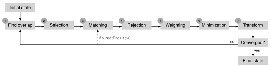
  • I: correspondences are established iteratively (i.e. not only once)
  • C: as correspondence the closest point, or more generally, the corresponding point, is used
  • P: correspondences are established on a point basis (instead of using e.g. interpolated surfaces or rasters)

The following flow diagram illustrates the functionality of this module. The main iteration loop consists of 7 main steps, which are described below.

Figure 1: Functionality of opalsICP.

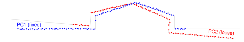
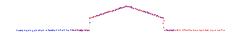
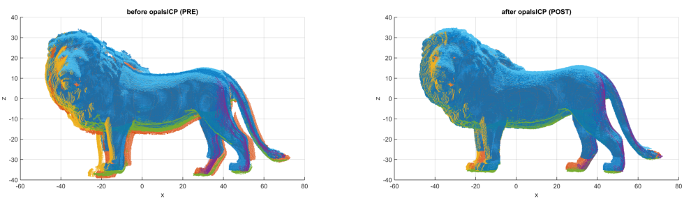
In the simplest case, the ICP algorithm is used to improve the orientation of a single loose point cloud with respect to a single fixed point cloud. The main steps of the algorithm are explained on the basis of this case. The initial orientation of the two point clouds is visualized in Figure 2. As can be seen, the point clouds are already roughly aligned, which is a main requirement of the ICP algorithm.

Figure 2: Initial state of the point clouds.

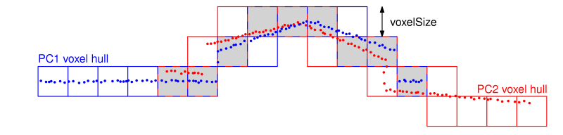
Step 1: Find overlap: The overlap area of the point clouds is determined by using so-called voxel hulls. Voxel hulls are a low resolution representation of the volume occupied by a point cloud. For the computation of the voxel hull the object space is subdivided into a voxel structure. The voxel hull of a point cloud consists of all voxels which contain at least one point of the point cloud. The parameter voxelSize defines the edge length of a single voxel.

Figure 3: Overlap area of the point clouds (grey filled voxels) as intersection of the two voxel hulls (blue resp. red voxels).

Step 2: Selection: A subset of points is selected within the overlap area in one point cloud. For this, points are first selected uniformly in object space, which leads to a homogeneous distribution of the points within the overlap area (uniform sampling). The mean sampling distance in each coordinate direction is defined by the parameter samplingDist. The selected subset of points can be further refined with the strategies normal space sampling or maximum leverage sampling, which are described in section Advanced selection strategies.

Figure 4: Selection of points in first point cloud.

Step 3: Matching: Find the closest points (= nearest neighbors) of the selected subset in the other point cloud. This step leads to a set of correspondences which possibly also includes some outliers.

Figure 5: Matching of the selected points (blue / from previous step) to the closest points (red) in the second point cloud.

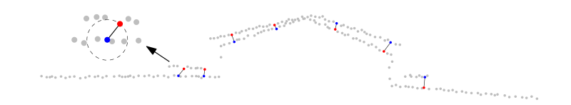
Step 4: Rejection: Rejection of false correspondences (outliers) based on the compatibility of points. Correspondences are rejected if:

  • the euclidean distance between corresponding points is larger than the value specified by the parameter maxDist.
  • the roughness attribute of one of the corresponding points is larger than the value specified by the parameter maxSigma. (Note: as roughness attribute the standard deviation in normal direction of the points used for plane fitting is used.)
  • the angle between the normals of corresponding points is larger than the value specified by the parameter maxAngleDev.

Since it is not guaranteed that with these strategies all outliers are rejected, a robust adjustment method is used in step 6 (Minimization) for the detection and deactivation of the remaining ones.

Step 5: Weighting: In this step a weight ( \(0 \le w \le 1\)) is assigned to each correspondence. Weights are based on:

  • the roughness attribute of corresponding points
  • the angle between the normals of corresponding points.

Step 6: Minimization: Estimation of the transformation parameters (for the loose point cloud) by a least squares adjustment. The adjustment minimizes the sum of squared point-to-plane distances. The point-to-plane distance of two corresponding points is defined as the orthogonal distance of one point to the fitted plane of the other point.

Figure 6: Minimization of the point-to-plane distances (green) between corresponding points.

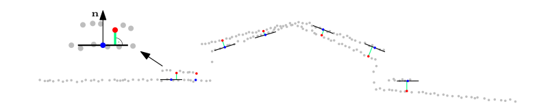
Step 7: Transformation: Transformation of the loose point cloud with the estimated parameters. The transformation model can be chosen with the parameter trafoType.

After step 7, a convergence criterion is tested. If it is not met, the process restarts with a new iteration from step 1 (Figure 1). However, if subsets are defined by the parameter subsetRadius, the iteration loop restarts from step 3 and the first two steps are only performed once. The total number of iterations heavily depends on the initial orientation of the points clouds, but typically, between 3 and 10 iterations should be sufficient to reach the global minimum.

Figure 7: Final state of the point clouds.

Note that opalsICP is not restricted to two point clouds, but can handle an arbitrary number of point clouds simultaneously.

Advanced selection strategies

The selection of points (step 2) can heavily affect the final alignment accuracy. Therefore, opalsICP offers two advanced selection strategies, which are especially useful for point clouds where one normal direction is predominating, but the data still includes some valuable features for the alignment. First, points are always selected with the uniform sampling strategy described above, where the mean sampling distance is defined by the parameter samplingDist. To select a subset of this selection, one of the two following strategies can be applied:

  • normal space sampling: The aim of this strategy is to select points such that the distribution of their normals in angular space is as uniform as possible. The percentage of points selected by this strategy can be defined with the parameter normalSpaceSampling.
  • maximum leverage sampling: This strategy selects those points, which are best suited for the estimation of the transformation parameters. For this, the leverage of each point on the parameter estimation is considered. The percentage of points selected by this strategy can be defined with the parameter maxLeverageSampling.

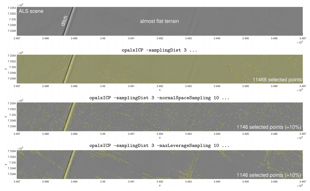
A comparison of the selection strategies offered by opalsICP is given in Figure 8. For most ICP variants, this ALS scene is rather difficult because only one feature - the ditch - can constrain the transformation at the finest level. Since normal space sampling and maximum leverage sampling consider the usefulness of points for the alignment process, the number of points can be dramatically reduced, without affecting the solubility of the adjustment. Further information can be found in Glira et al. 2015.

Figure 8: The advanced methods 'normal space sampling' and 'maximum leverage sampling' for the selection of points (step 2).

Parameter description

Note that the default parameter values were chosen to be well suited for ALS point clouds. For point clouds at other scales, the Examples section may serve as a reference.

-inFilelist of input files
Type: opals::Vector<opals::Path>
Remarks: mandatory
The input files containing the unregistered point clouds (i.e. individual scan positions, flight strips...) can be provided in any OPALS supported Format. If not OPALS Data Manager (ODM) format is used, the reduction point currently has to be stated explicitely using -redPoint. Note that wildcard characters (*,?) can be used for the selection of multiple files at once (e.g. scan*.odm).
-redPoint3d coordinate reduction point
Type: opals::Array<double, 3>
Remarks: estimable
The reduction point defines the origin of a local coordinate system in which the point clouds are stored internally - for different input formats than ODM, this parameter is mandatory. Using a reduction point is crucial for large coordinates, since otherwise transformation parameters are highly correlated.
Estimation rule: Use the center of gravity of the bounding boxes of all input ODMs.
-filtermodify the input using a (tree of) filter(s)
Type: opals::String
Remarks: optional
A filter string in EBNF syntax as described in section 'Filter syntax' can be passed to restrict the set of input points used within the ICP algorithm (e.g. only last echoes or only smooth areas). Note that this parameter does not affect the final ODM files in which (regardless of the filter settings) always all points are included.
-outDirectoryoutput directory
Type: opals::Path
Remarks: mandatory
To specify the folder where the final transformed datset files and additional log and MATLAB files are stored. Note that the transformed datasets are only generated if transformData is activated and that they are furthermore created in the same data format as the input files.
-tempDirectorytemporary data directory
Type: opals::Path
Remarks: default=tempICP
To specify the folder where temporary data are stored (e.g. intermediate MATLAB files).
-trafoTypetransformation type
Type: opals::LSMTrafoType
Remarks: default=full
Possible values:  
  zShift .... compute z-shift only
  shifts .... compute 3D-shifts only
  rigid ..... compute rigid 3D transformation (3 rotations + 3 shifts = 6 parameters)
  helmert ... compute 3D Helmert transformation (3 rotations + 3 shifts + 1 scale = 7 parameters)
  full ...... compute full 3D affine transformation (12 parameters)
Allows to specify the transformation model applied to the point clouds within the ICP algorithm.
-fixedFilefile name(s) of fixed point cloud(s)
Type: opals::Vector<opals::Path>
Remarks: estimable
In order to define the datum of the adjustment, at least one point cloud has to be fixed in object space. With this parameter the file names of one or more fixed point clouds can be defined.
Estimation rule: If not specified, the first inFile is fixed.
-voxelSizevoxel size of voxel hulls
Type: double
Remarks: default=10
The edge length of a single voxel used for the voxel hull computation to detect overlaps. 100 must be a whole multiple of it: fmod(100,x) == 0.
-samplingDistmean distance between corresponding points
Type: opals::Vector<double>
Remarks: default=10
The selection of correspondences is based on a 3d uniform sampling strategy. This parameter defines the mean sampling distance in each coordinate direction. In the case that more than one value is passed, specific sampling distances are used for the n individual input datasets (-inFile). If less than n values are specified the last value is used for the remaining datasets.
-searchRadiussearch radius for plane fitting
Type: double
Remarks: default=2
The implemented ICP algorithm minimizes point-to-plane distances i.e. points in one point cloud are compared to planes in all overlapping point clouds. All points within a sphere of the specified radius are considered for the plane fitting. A good choice of the search radius is based on the point cloud density and the geometry of the scanned object. Note: to ensure a certain redundancy, planes are only considered if the search area contains at least 8 points.
-maxItermaximum number of iterations
Type: int32
Remarks: default=5
Maximum number of iterations within the ICP algorithm.
-subsetRadiusradius of selected subset areas
Type: double
Remarks: default=0
For large point clouds (e.g. ALS flight block), it is usually not possible to load all point clouds in memory simultaneously. Thus, only a small subset of points is selected for each point cloud. For this points are selected around the established correspondences within a specific radius defined by this parameter. If subsets are used, the main iterations loop restarts from step 3 instead of step 1 (Figure 1), i.e. step 1 and step 2 are only performed once. This parameter can be set to zero if no subsets should be used, i.e. all point clouds can be kept in memory simultaneously.
-maxDistmaximum distance between corresponding points
Type: double
Remarks: estimable
To reject false correspondences, a maximum allowed (point-to-point) euclidean distance between two corresponding points can be defined with this parameter.
Estimation rule: 2*searchRadius.
-maxSigmamaximum plane roughness
Type: double
Remarks: default=0.1
To reject false correspondences a maximum allowed roughness value (i.e. standard deviation of plane fitting) can be defined with this parameter. This way the ICP algorithm only considers smooth surfaces for estimating the transformation parameters. Whenever possible, a small threshold should be used to ensure high-quality correspondences. Higher values, in turn, increase the number of correspondences.
-maxAngleDevmaximum angle (in degrees) between the normals of corresponding points
Type: double
Remarks: default=10
To reject false correspondences, a maximum deviation between the angles of normals of two corresponding points can be defined with this parameter.
-normalSpaceSamplingpercentage value for normal space sampling
Type: double
Remarks: optional
Normal space sampling is an advanced selection strategy which can be used to reduce the points previously selected by the parameter samplingDist. This parameter defines the percentage of the remaining points.
-maxLeverageSamplingpercentage value for maximum leverage sampling
Type: double
Remarks: optional
Maximum leverage sampling is an advanced selection strategy which can be used to reduce the points previously selected by the parameter samplingDist. This parameter defines the percentage of the remaining points.
-plotvisualization of ICP results
Type: bool
Remarks: default=0
If specified, after each ICP iteration a 3d point cloud visualization and the most relevant ICP results are displayed in a window.
-transformDataperform input data transformation
Type: bool
Remarks: default=1
If activated, the estimated transformations are applied to each individual input data set. The resulting ODM files are stored in the folder specified by the outDirectory parameter (subfolder post).
-outTrafParsoutput transformation parameters
Type: opals::Vector<opals::TrafPars3dAffine>
Remarks: output
The results of the ICP computation are the transformation parameters for each input dataset.
TrafPars3dAffine: Describes a relative or absolute 3D-affine transformation. This class contains the transformation parameters of an affine 3D (i.e. 12-parameter) transformation, given as 12-array

Examples

The data used in the following examples can be found in the $OPALS_ROOT/demo/ directory.

Example 1: ALS strip adjustment

In this example a small strip adjustment (3 strips) is calculated with opalsICP. Besides the mandatory parameters inFile and outDirectory, we also set the samplingDist to 5m and the reduction point (redPoint) since we are directly using LAS data:

opalsICP -inFile G111.las G112.las G113.las -outDirectory icpALS -samplingDist 5 -redPoint 2000 338900 0
Figure 9: Results obtained with opalsICP (set the parameter plot to true for this visualization).

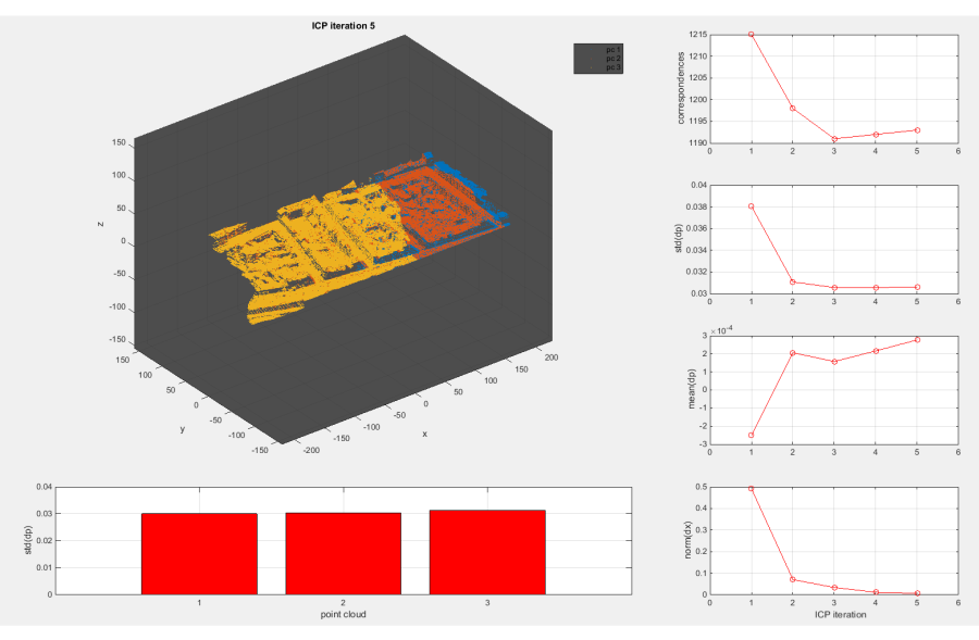
Please note, that all values displayed in this visualization are also included in the command line output:

B | S : GLOBALICP > RUNICP > ICP ITERATION 5 OF 5 > RESULTS
B | T : -------------------------------------------------------------------------------
B | T : GENERAL STATISTICS:
B | T :    iteration     corresp.      std(dp)     mean(dp)     norm(dx)
B | T :            1         2422      0.04827      0.00189      6.42463
B | T :            2         2369      0.03621      0.00070      5.78050
B | T :            3         2363      0.03632      0.00073      0.94349
B | T :            4         2365      0.03605      0.00074      0.29409
B | T :       new: 5         2362      0.03611      0.00075      0.11907
B | T : where dp = vector of all (signed) point-to-plane distances
B | T :       dx = vector of parameter increments
B | T : -------------------------------------------------------------------------------
B | T : POINT CLOUD DEPENDANT STATISTICS:
B | T :  point_cloud     corresp.      std(dp)     mean(dp)     file
B | T :          [1]         1121      0.03689      0.00034     G111
B | T :          [2]         2059      0.03478      0.00087     G112
B | T :          [3]         1544      0.03726      0.00090     G113
B | T : where dp = vector of all (signed) point-to-plane distances associated to a single point cloud
B | T : -------------------------------------------------------------------------------
B | E : GLOBALICP > RUNICP > ICP ITERATION 5 OF 5 > RESULTS

The following files are created in the folder specified by the parameter outDirectory:

  • Final (not filtered) transformed point clouds in LAS file format:
    icpALS\G111.las
    icpALS\G112.las
    icpALS\G113.las
    
  • Command line output (also contained in opalsLog.xml):
    icpALS\ICPLog.txt
    
  • ICP result file for further analysis in Matlab:
    icpALS\ICP.mat
    

The following files are created in the temporary folder (not explicitly specified in the above command):

  • (Filtered) input point clouds in mat format:
    tempICP\G111.mat
    tempICP\G112.mat
    tempICP\G113.mat
    
    These point cloud files correspond to the LAS file format and can be opened in MATLAB (as objects of class pointCloud).

Please note that the transformed output files (icpALS\*.las) are exported in the same data format (LAS version, point data record format) as the input LAS files. Please use Module Import to convert the LAS files to OPALS Datamanager format for further use within OPALS.

Example 2: Close range TLS dataset

In this example the orientation of six overlapping close range TLS scans is improved by opalsICP. The initial orientation of the scans is shown on the left-hand side of Figure 10 (coordinate units = mm). Please note: since the default parameter values of this module were chosen to be well suited for ALS point clouds, compared to the previous example, a few more parameters have to be specified:

opalsICP -inFile lionScan1.las lionScan2.las lionScan3.las lionScan4.las lionScan5.las lionScan6.las -outDirectory icpCloseRange -samplingDist 4 -searchRadius 2 -maxSigma 0.5 -trafoType rigid -redPoint 0 0 0
Figure 10: The orientation before and after running opalsICP.

The new OPALS Datamanager files are placed in the folder icpCloseRange.

Example 3: TLS dataset

The orientation of three TLS scans of a room is improved in this example. As a first step, the data are imported to ODM format:

opalsImport -inFile roomScan1.laz -outFile roomScan1.odm
opalsImport -inFile roomScan2.laz -outFile roomScan2.odm
opalsImport -inFile roomScan3.laz -outFile roomScan3.odm

The following call of opalsICP differs from the previous examples in two points:

  • A wildcard character is used to define the list of input files.
  • The input data is not transformed within opalsICP, which means that no ODM files are created in the folder icpTLS. Instead, the transformation parameters are written to the file icp_output.xml. This file can afterwards be used to directly transform the input data into any format supported by OPALS.
opalsICP -inFile roomScan?.odm -trafoType rigid -voxelSize 0.2 -samplingDist 0.5 -searchRadius 0.1 -maxSigma 0.02 -outDirectory icpTLS -transformData false -outParamFile icp_output.xml
Figure 11: A cross-section through the scanned interior before and after running opalsICP.

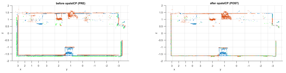
Now, we can directly create the transformed LAS files with Module Export using Parameter Mapping to set the transformation parameters trafo:

opalsExport -inFile roomScan1.odm -outFile icpTLS\roomScan1.las -inParamFiles icp_output.xml -paramMapping "trafo = opalsICP.outTrafPars me.inFile[0].stem().startswith( Path(you.getIdGridMov()).stem() )"
opalsExport -inFile roomScan2.odm -outFile icpTLS\roomScan2.las -inParamFiles icp_output.xml -paramMapping "trafo = opalsICP.outTrafPars me.inFile[0].stem().startswith( Path(you.getIdGridMov()).stem() )"
opalsExport -inFile roomScan3.odm -outFile icpTLS\roomScan3.las -inParamFiles icp_output.xml -paramMapping "trafo = opalsICP.outTrafPars me.inFile[0].stem().startswith( Path(you.getIdGridMov()).stem() )"

References

Besl P., McKay N., 1992. A Method for Registration of 3-D Shapes. In: IEEE Trans. PAMI, Vol. 14, No. 2: 239-256.

Chen Y., Medioni, G., 1991. Object Modeling by Registration of Multiple Range Images. In: Proc. IEEE Conf. on Robotics and Automation, Sacramento, California: 2724-2729.

Glira P., Pfeifer N., Briese C., Ressl C., 2015: A correspondence framework for ALS strip adjustments based on variants of the ICP algorithm.

Author
pg, gm, jo, mw
Date
11.11.2018
@ redPoint
defines the coordinates of a reduction point
@ transformData
boolean flag indicating whether or not to transform the input data (eg. opalsICP)
@ outParamFile
final parameter export
@ paramMapping
mapping of parameters from file to own parameters
opalsImport is the executable file of Module Import
Definition: ModuleExecutables.hpp:113
@ samplingDist
defines a uniform sampling distance (eg, opalsICP)
opalsExport is the executable file of Module Export
Definition: ModuleExecutables.hpp:73
@ inParamFiles
parameters to import from file
@ trafoType
transformation type (opalsICP)
opalsICP is the executable file of Module ICP
Definition: ModuleExecutables.hpp:108
@ rigid
compute rigid 3D transformation (3 rotations + 3 shifts = 6 parameters)
@ outDirectory
name of output directory
@ voxelSize
defines the size (edge length) of voxel cube)