Technische Universität Wien
Orientation and Processing of Airborne Laser Scanning data
Department of Geodesy and Geoinformation - Research Groups Photogrammetry and Remote Sensing
Supervised classification based on machine learning allows classifying unseen data based on models that have been trained on a small, representative set of training data. The provided solution in OPALS utilises CART (Classification and regression trees) modelling as implemented in the software package R.
The concept uses individual point classification, meaning that each point is classified separately based on its coordinates and attributes without considering its neighbourhood. However, the neighbourhood of a point generally contains important implicit information that is useful for many applications. This is why, local point distribution measures like normal vector, surface roughness, vertical point distribution, point density, etc. need to computed and assigned as attributes to each point to achieve good classification results. The more distinctive those attributes are regrading sought-after classes, the better the classification accuracy will be. Calculating appropriate features within an adequate neighbourhood area is therefore a crucial pre-processing step as described in the attribute computation section. The training of the tree model and its evaluation is described in the training section, whereas utilisation of the trained model to classify unseen data can be found here. At the end of this page, a classification example is shown.
The tree based classification method requires an R installation including the lasr package. See here for installation details.
As mentioned above, the computation of significant point attributes is crucial for achieving good classification results. Modules that extract information from the point cloud and add them as attributes to each point are Module Normals, Module EchoRatio, Module PointStats, and Module AddInfo. For convenience reasons, OPALS provides a script that allows computing attributes in a flexible and unified way. preAttribute.py performs a sequence of module calls for a specified list of input files in two different modes:
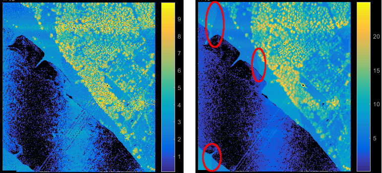
In file-wise processing mode, the input files are directly passed to the corresponding modules, whereas for strip-wise processing the script virtually splits each input file into their original strips (using filters). This requires the existence of a strip identifier attribute (e.g. PointSourceId as defined in the LAS standard) that was correctly set during import. The strip-wise processing mode is useful for features that should not be effected by strip overlaps. In case of ALS and homogeneous scan pattern (perpendicular to the flight direction), the point density e.g. reflects penetrable regions (=multi-target regions) providing a good indicator for vegetation. Not considering strip overlaps would naturally downgrade this vegetation measure (see Figure 1). On the other hand, for other attribute extraction steps the increase of information within the overlapping areas are desired.
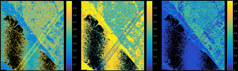
Surface roughness, normal vector and local structure tensor features are important and significant attributes for the point classification. Module Normals provides the central computation functionality for those features. Based on the given neighbourhood definition and adjustment method, local surface normals are computed, which deliver the surface roughness (attribute NormalSigma0) and the structure tensor as a by-product. Adapting parameter storeMetaInfo for Module Normals the eigenvalues and eigenvectors of the structure tensor are attached as attributes to each point. Using Module AddInfo, further measures (e.g. linearity, planarity, omni-variance, etc.) can be derived as shown in Figure 2. For further details, please refer to the reference section below.
More details on the preAttribute script can be found here.
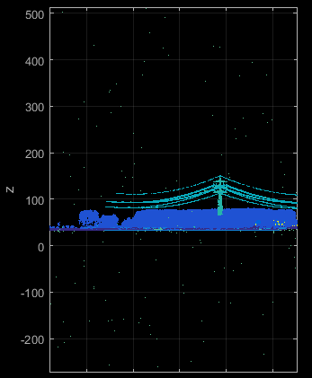
Raw point clouds from ALS or dense image matching usually contain outliers. Their characteristics and amount differ based on the measurement principle and sensor. However, any gross error will distort the attribute computation in its vicinity (especially attributes that are computed within a 2D neighbourhood). In ALS such outliers are often called long or short ranges, since they are obviously not reflected from either the bare Earth or from any other natural (vegetation) or artificial (buildings, power lines) target (see Figure 3).
Although it is also possible to train the classification to detect outliers, practical tests have shown that classification accuracies are usually better for point clouds where outliers have been removed in advanced. It turns out that inliers within the local neighbourhood of long ranges are often labelled incorrectly, although the overall classification accuracy only slightly decreases. This effect can be analysed by the user since the demo data shown below do contain (classified) outliers.
A detailed discussion on efficient outlier detection is omitted here. Basically detecting isolated points (using Module AddInfo) and applying a coarse DTM and DSM can solve this task.
Any supervised classification method requires training data, which are used by the machine learning algorithm to build the classification model. In general, only a certain part of the available data are used for the actual training. The remaining data are then used for cross validation of the trained model allowing to estimate the accuracy of the created model.
As mentioned above, OPALS utilises CART modelling via the rpart (acronym for Recursive PARTitioning) package of the open source R-project for statistical computation. The classify scripts calls the rpart functions indirectly through the lasr package. For details on the rpart routines please refer to this introduction).
For the training stage, three central inputs are required:
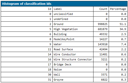
It is not necessary that all points of the input file(s) have been labelled, but all classes must occur in the training dataset as the model cannot be trained for non-existing classes. The distribution of the class labels should roughly match the label distribution in the files that should be classified since this information is used to build the classification trees. Therefore, the clfTreeModelTrain script computes a label histogram for all input files.
If class labels are not covered in the training data, the script stops with a corresponding error message (or outputs a warning if the OmitEmptyClasses flag is activated).
In the next step the corresponding training subset is transferred to R to perform the actually training. As mentioned above, it is important to only use a subset for training (and the remaining data for cross-validation). The subset percentage can be defined by parameter TrainingSize. Setting an appropriate value is crucial in terms of multiple aspects:
Considering the aforementioned, the training size should be as small as possible (faster computation, higher significance of cross-validation) but large enough to build a robust classification model. A good indicator for large enough training sizes is given by running the train script multiple times. Since the script always randomly sub-selects the training data, each run will lead to (slightly) different results. If the overall accuracy and the confusion matrix doesn't change significantly, the training size can be considered large enough.
As for other package scripts, only basic parameters (-i input files, -c configuration file, -o output directory) can be directly passed to the script. All other parameters need to be set by a configuration file in the [script.clfTreeModelTrain] section.
If the training succeeded, the tree model is saved to file as defined by the classificationModel parameter. Changing this parameter allows creating different models for later usage.
At the end of the cross-validation stage, a confusion matrix is printed. This is a quantitative comparison of the reference classes to the estimated classes obtained from the trained model. The rows of the matrix represent the reference classes whereas columns describe the estimated class labels.
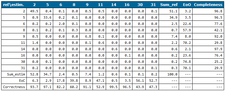
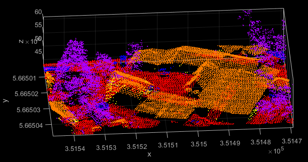
The confusion matrix reveals classes that can be estimated well (w.r.t. completeness and correctness) and problematic ones by checking EoO (Error of Omission) and EoC (Error of Correctness). E.g. in the Niederrhein example (see Figure 5) the completeness of class 11 (Road Surface), 30 (Walls) and 31 (Groyne) is below 30%. Estimated road surface points (see column 11 in Figure 5) are either ground (class 2), water (class 9) or road surface points (class 11). This is not surprising since all three classes do have very similar geometry properties (smooth flat region). The differentiation is based on the calibrated reflectance attribute which obviously doesn't perform well enough. The situation is similar for groynes (class 31) which is why ground points are also labelled as class 31. Their distinctive property that they are surrounded by water is not described by any of the used attribute features. The poor quality of wall points is evident when inspecting those points visually. The point density of this dataset is simply not high enough and the buildings are too low, respectively, that walls are properly captured by the laser scanner (see Figure 6).
Finally, it should also be mentioned that the confusion matrix is also printed with absolute numbers to the OPALS log with log level verbose. This helps analysing classes that have a very low relative frequency.
Due to the lack of an interactive 3D point cloud editor, it is currently not possible to visually create training data within OPALS. However, several commercial and open source software packages (e.g. MeshLab, CloudCompare, etc.) exist for this task. The labelled point cloud can then be directly processed with the preAttribute and clfTreeModelTrain script or the point labels are merged back into the existing ODM files (cf below for more details).
After a satisfactory model has been trained, the model can be applied to classify the unseen data. First, the preAttribute script has to be used for processing all data files (if not done already) with exactly the same configuration file as for the training data. ATTENTION: This is not checked by OPALS and can lead to wrong classification results if different parameters are applied. Finally, the clfTreeModelApply script can be started with a corresponding configuration file that has two main parameters:
For completeness it is mentioned that the rpart algorithm can handle missing attribute values (e.g. normal estimation can fail because of a lack of neighbours) whereas other tree classifier usually exclude such data from processing.
All data used in the following examples are located in the $OPALS_ROOT/demo/classify directory of the OPALS distribution. The three commands in the section below perform a full classification workflow including:
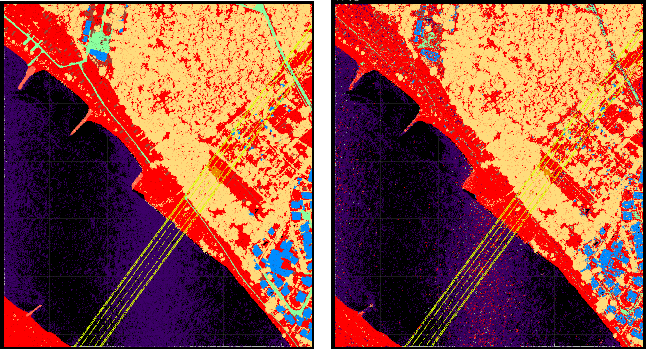
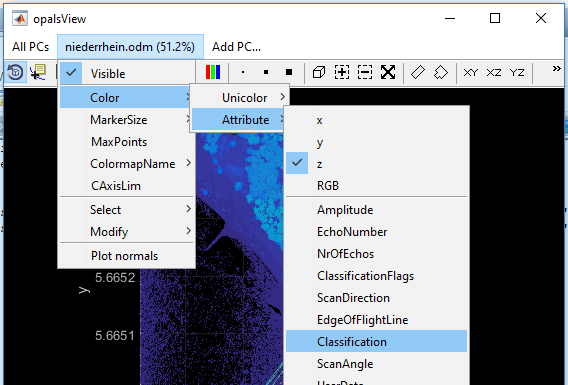
preAttribute)clfTreeModelTrain)clfTreeModelTrain)After running the above commands, the resulting niederrhein.odm file contains the reference and estimated class labels (attribute classification and _classEstim). Module View allows a visual inspection of the class labels using attribute colourization (see Fig 8) and color map name classpal.
B. Madsen, U.A. Treier, A. Zlinszky, A. Lucieer, S. Normand, S.: Detecting shrub encroachment in seminatural grasslands using UAS LiDAR, Ecol Evol. 2020; 00: 1 - 27. https://doi.org/10.1002/ece3.6240
J. Otepka, S. Ghuffar, C. Waldhauser, R. Hochreiter, N. Pfeifer: Georeferenced Point Clouds: A Survey of Features and Point Cloud Management, ISPRS International Journal of Geo-Information, 2 (2013), 4, 1038 - 1065.
C. Waldhauser, R. Hochreiter, J. Otepka, N. Pfeifer, S. Ghuffar, K. Korzeniowska, G. Wagner: Automated Classification of Airborne Laser Scanning Point Clouds, Solving Computationally Expensive Engineering Problems, Volume 97 of the series Springer Proceedings in Mathematics & Statistics; S. Koziel, L. Leifsson, X. Yang (ed.); Springer, 2014, ISBN: 978-3-319-08984-3, 269 - 292.
 1.8.17