Technische Universität Wien
Orientation and Processing of Airborne Laser Scanning data
Department of Geodesy and Geoinformation - Research Groups Photogrammetry and Remote Sensing
Derives histograms and descriptive statistics (min, max, mean, r.m.s, etc.) for ODM or grid/raster data sets and stores the results graphically (SVG) and numerically (XML).
Data analysis is of crucial importance for ALS data processing. Besides 3D views and 2D maps, histograms of specific data attributes (including standard statistical parameters) are useful tools for analyzing certain data characteristics (e.g. distribution of heights, amplitudes, return numbers, gradients...) and for checking the data quality (e.g. strip differences considered to be normally distributed with expectation value = 0). Whereas 2D maps visualize the spatial distribution of certain data attributes, histograms condense the entire information in a bar plot and the descriptive statistical measures summarize and characterize the whole data sample. Thus, decisions upon the necessity of additional processing steps (e.g. strip adjustment) no longer rely on a pure visual data inspection but they are supported (or even advised) by quantified statistical measures. The following statistical parameters are provided:
Module Histo operates on either vector data sets (OPALS Data Manager, ODM) or regular grids/rasters in GDAL supported data formats. In both cases a single or multiple input files (of the same type) can be specified (parameter inFile). By default, the histograms and statistics are calculated for the heights (z) of the ODM point cloud or the first band of the grid/raster dataset, respectively. However, any other attribute stored in the ODM (as additional info) or raster band (zero-based band index or band name) can as well be used as basis (parameter attribute). In case of several user-selected attributes, the module derives seperate histograms and statistics for each attribute or raster band. The respective data samples are sorted into bins (classes) of equidistant width. The width can be specified either explicitly by a specific bin width (parameter binWith), or implicitly by the desired number of different bins (parameter nBins, default: 20). By default, the histogram is limited to the 0.02 and 0.98 quantile moving (possible) outliers to the underflow and overflow bin. This behavior can be changed with the sampleRange parameter, by specifying relative or absolute sample range values. Relative values can be either specified in percentage (e.g. 5%) or in quantile (e.g. q:0.05) notation. Please note that the quantiles are by default only approximated, which may result in slightly incorrect histogram limits, as shown in Figure 1. If exact limits are required the exactComputation mode has to be activated. If the histogram should cover the full sample range from \(x_{min}\) to \(x_{max}\) (without underflow and overflow bins), one can either specify quantile 0 and 1 (-sampleRange q:0 q:1) or use the min max labels (-sampleRange min max). See example 3 for further details.
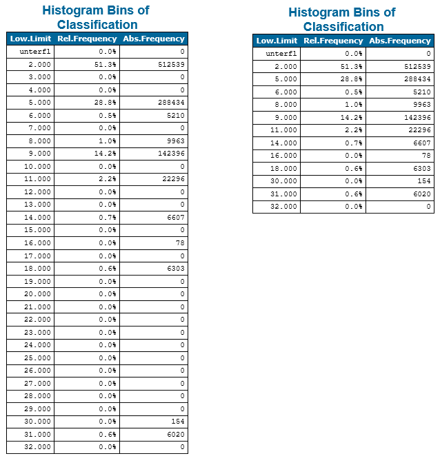
For processing integer attributes (EchoNumber, Classification, etc.) the module provides a specific integer processing mode (see procMode) where the bin width is constraint to integer values. Furthermore, the bin borders are shifted by half of the bin width, so that the bin centers correspond to the integer values (see EchoNumber histogram in Figure 1). By default the module automatically switches to real or integer processing mode based on the type of the ODM attribute or the raster band type. Nevertheless, this behavior can be overruled by the procMode parameter. For non-continuous attributes like classification values, it might be relevant to skip empty bins (see parameter skipEmptyBins) within the histogram (see example 5).
To limit the memory consumption, the module uses several approximation strategies that avoids storing all values in a sorted vector or list. Using the extended \(P^2\) algorithm (Jain and Chlamtac, 1985) for estimating quantiles and three data passes the median and sigma(mad) can be computed with a decent precision. Nevertheless, in certain siutation the exact quantiles, median and sigma(mad) values are required. This can be achieved by activating the exact computation mode (parameter exactComputation). There, the complete data series needs to be stored in a sorted vector, which might not be possible for huge data sets. On the other hand, the exact computation mode only requires one data pass which is typically faster than the non-exact mode. In case the module cannot allocate the vector for the full data series, it automatically drops back to the non-exact mode and outputs a warning.
Unless otherwise specified, all available data are considered for the calculations. However, in some situation it might be advantageous to restrict the input data. This can be achieved by specifying a data window (parameter limit) and/or a selection condition (parameter filter). The filter string must correspond to the OPALS Filters syntax. Please note, that filters based on certain point attributes (e.g.: Echo, Class, ...) are not practicable for grid/raster datasets as the 3D grid points (x,y, grid value) do not contain additional point attributes. It is advisable to use the limit parameter (e.g.: limit xmin ymin xmax ymax) to specify a specific data window rather than specifying a region filter (e.g.: parameter filter "Region[xmin ymin xmax ymax]"). In the latter case the region filter is applied to the entire dataset (all ODM data points or entire grid) whereas in the first case a spatial sub-selection is applied beforehand resulting in better program performance. This is especially important when statistics are to be derived for a series of small patches based on the same data set using Module Histo repetitively. It is even possible to combine limits and filters in which case, first, the window query is applied and, subsequently, all points within the window area are checked w.r.t. a (potentially more complex) region filter polygon.
Finally, the results (histogram and statistics) are stored as a complex object separately for each attribute. For the Python and C++ class implementations the results are directly accessible for further use (e.g. to decide on further processing steps based on statistical measures). Beyond that, graphical output (parameter plotFile) is provided as Scalable Vector Graphics which can be displayed in standard web browsers (Firefox, Opera, IE...). If an output parameter file (parameter outParamFile) is specified, the (numerical) results are additionally written to an XML file.
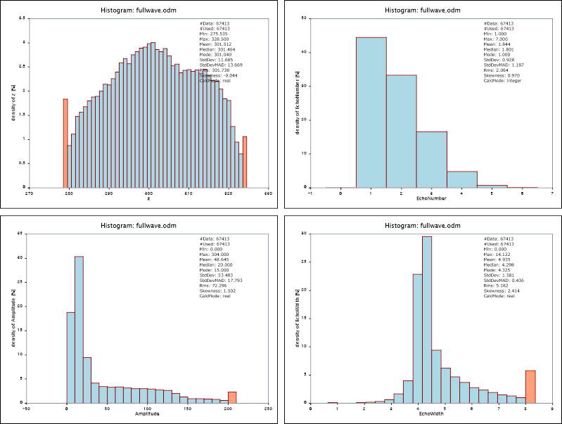
The data used in the following examples are located in the $OPALS_ROOT/demo/ directory. Example 1 shows several histogram variants based on an ALS point cloud (fullwave.odm) whereas example 2 features histograms of regular grids (stip19/20.tif).
As a prerequisite for the following example, the ALS point cloud data must be imported into the ODM. To achieve that, change to the demo directory and type:
Now, we are ready to derive histograms based on the resulting ODM featuring the 3D-coordinates (x, y, z) and additional attributes (x, y, z, gps time, amplitude, echo width, echo nr, echo qualifier) for each point. The following example demonstrates how to to analyze different point attributes in the form of histograms:
The following SVG plot files are created:
Please note, that the names of the respective SVG plot files (not specified explicitly in the above examples) have been estimated from the input file and attribute names. The results are shown in Figure 1.
A numerical representation of the histogram and statistics can be obtained by specifying an output parameter file as shown in the first example (parameter outParamFile). The resulting XML file histo.xml contains the following output (excerpt):
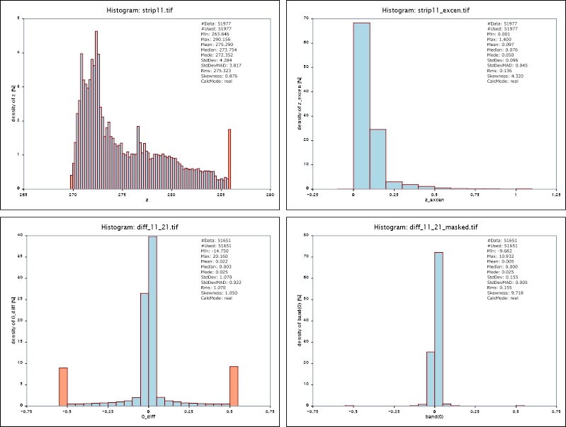
Example 2 shows how to derive histograms of grid datasets. To generate the underlying grids, please perform the following preprocessing steps:
This procedure, first, imports the data of strips 11 and 21 (strip11/21.las) into separate ODM files, and generates surface models as well as additional "sigmaZ" (=smoothness) and "excenter" (=extrapolation/occlusion) layers for each strip (strip11.tif, strip11_sigmaZ.tif, strip11_excen.tif). Subsequently, a strip difference model (diff_11_21.tif) and a respective grid mask (diff_11_21_mask.tif) are derived. The examples below (results c.f. Figure 2) show the distribution of the grid heights and excenter layer of the surface model of strip 11. Furthermore, the height differences between strip 11 and 21 are analyzed in two variants, one using all available height differences in the strip overlap area, an the other one considering a grid mask to exclude all rough and occluded pixels.
Please further note, that wild cards are supported in case of multiple input datasets.
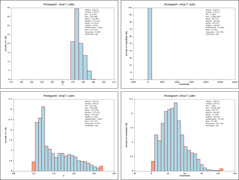
By default the module uses the 2% and 98% quantile to limit the histogram. This typically moves outliers to the underflow and overflow bins and presents the relevant data with appropriate resolution. The follow example shows the effect on the z and amplitude attribute for demo dataset strip11.
Since the dataset contains long ranges and high amplitude values, the full range histograms are not very meaningful (upper images of figure 3) whereas the distribution of the attributes is nicely visable using the standard sample range (lower images of figure 3)
The main benefit of running Module Histo in Python is that the histogram as well as all standard statistics (min, mean, median, ...) are directly accessible after running the module via the Python API. This is exemplified in the sample script $OPALS_ROOT/demo/histoDemo.py:
To run the script, type:
The script queries the output parameter histogram provided by Module Histo as a complex Python type (class) and uses its access functions to print the min, median, and 95% height quantile of the dataset <fullwave.odm>. The following output is printed to the screen:
Example 5 demonstrates the skipEmptyBins parameter and its effect on the histogram. For non-continuous (integer) attributes like classification values or the like, a continuous histogram that covers the full data range might be inappropriate since the magnitude of those values is typically irrelevant. Activating the skipEmptyBins parameter as shown below, only plots occupied bins next to each other despite of the bin borders. To make non-continuous histogram easily recognizable, a uniform gab between all bars are inserted.
The skipEmptyBins parameter not only influences the visual presentation of the histogram but also the actual bin table within the OPALS log as well as the python histogram object.
With a few lines of python code it is straightforward to generate a Q-Q plot. Plotting quantiles of a theoretical distribution against computed quantiles of a data set, the equality of the two probability distributions can be visually analyzed. In this example the height differences of strip11 and strip21 (as computed above and written to file diff_11_21.tif) are compared against the normal distribution. Run the Q-Q-plotDemo.py demo script with the following parameters
to see figure 6 on the screen. When generating Q-Q plots it is recommended to compute exact quantiles by activating the exactComputation parameter (see General description).

Sometimes it is of interest to see if the values of a given sample follow a certain theoretical distribution like the normal one. In this example, we will check if the difference of the strips strip11 and strip21 follow the normal distribution. For this, we will limit the analysis to smooth objects, like streets or roofs, because the differences at rough objects, like (high) vegetation, will not obey the very same distribution. We assume grid cells to be smooth if sigma0 of their moving planes interpolation is below 10 cm, which is realised using a mask.
Figure 7 below shows the color coded masked strip difference, limited to smooth areas.

With the following command the histogram of these differences is plotted together with the theoretical normal distribution based on the mean and the standard deviation derived from these differences, which are -0.009 m and 0.309 m, respectively.
Figure 8 (left) shows the result and one can clearly see, that the density curve of the normal distribution based on mean and the standard deviation from sample do not fit together at all. The reason for this is visible in figure 7. Some smooth cells have very large differences, which obviously do not belong to the same distribution as most of the other smooth cells. These outlier cells mostly appear at moving objects on the streets where e.g. in one strip the street surface is measured whereas in the other strip at the very same location the roof of a car was measured. In order to exclude these outliers from deriving the defining parameters of the normal distribution, one either has to fine-tune the mask (e.g. by manual inspection and correction) or one simply uses robust statistics. For the normal distribution, the median is a robust estimate of the mean and the MAD-based standard deviation is a robust estimate of the standard deviation. Using these values, which are -0.050 m and 0.011 m, as defining parameters for the theoretical normal distribution in the opalsHisto call is done in the following way:
Figure 8 (right) has the result, which clearly shows that the theoretical normal distribution based on these robustly estimated values represents the strip differsence very well.

The cumulative histogram can be useful to (roughly) estimate quantiles of a given sample. In this example we'll compute the point density (based on last echoes) for the strip11.
Which point density is provided by the data of strip11? In order to answer that question, one has to derive a certain statistic. For this the histogram can be useful:
The resulting histogram with the cumulative version is shown in figure 9.

In an heuristic approach one could use the derived median (6.75 points/ \(m^2\)) and say that the point density of strip11 is roughly 7 points/ \(m^2\).
The density palette for color coding is motivated by the traffic light paradigm: green indicates ok, yellow means attention, and red indicates stop. Consequently, the color coding of the point density of strip11 using 7 points/ \(m^2\) as reference value
would look like:

Judging by the large areas colored in yellow, orange and red, this data, obviously, does not provide 7 points/ \(m^2\) everywhere. Actually, since the color coding is based on the median value, only 50% of the area will appear in green tones.
Figure 10 clearly shows, that the point density in this section of this strip (which was flown roughly in south-east direction) is not homogenous. One can see scan shadows close to the buildings and two larger regions with low density (in yellow and orange color, respectively) orthogonal to the flight direction. The latter low density areas are caused by aircraft motions (e.g. wind-induced pitch variations).
Because of these density variations, one cannot expect the same point density everywhere. Consequently, one must be tolerant and willing to accept a certain portion of the area to be less dense. And this is where quantiles are helpful. If we are asking for the point density that is guaranteed in e.g. 95% of the area, i.e. we are willing to accept 5% of low density, then we ask for the 0.05 quantile (or 5-th percentile). Using the cumulative histogram in figure 9, these quantiles can be roughly estimated: Following the red line the 0.05 quantile is roughly 3 points/ \(m^2\). If we would be willing to accept 10% of low density, then the 0.10 quantile would be around 4 points/ \(m^2\) (indicated by the green line in figure 9).
In case of an accepted low density portion of 5% the color coding would look like:

The prevailing green tones in this color coding reflect our choice that 95% of the area guarantees 3 points/ \(m^2\).
By the shape of the cumulative histogram we also get an idea of how critical our choice of the acceptable low density portion is.
Addendum: If we know right from the beginning, that we will only tolerate a low density portion of e.g. 3%, then we can call opalsHisto with the probabilities parameter:
In this case it might by good to initiate the exactComputation mode instead of the default approximate computation. The differences in this example are small:
Ressl, C., Kager, H. and Mandlburger, G., 2008. Quality checking of ALS projects using statistics of strip differences. In: IAPRS, XXXVII, pp. 25399860.
R. Jain and I. Chlamtac, The \(P^2\) algorithm for dynamic calculation of quantiles and histograms without storing observations, Communications of the ACM, Volume 28 (October), Number 10, 1985, p. 1076-1085.
 1.8.17