Provides methods for point cloud segmentation based on local homogeneity using either a generic region growing approach or an adapted region growing for plane extraction.
As the single points in the point cloud do not contain information about the connectivity and structure of scanned objects, segmentation is needed to group points with similar properties. This module provides two different segmentation methods, that are both based on the seeded region growing approach. In both segmentation modes, a proper homogeneity criterion allows to detect segments for objects of interest.
The used seeded region growing approach works as follows (see Figure 1):

The point cloud is read from an OPALS Data Manager (ODM) input file (parameter inFile). Because of the tile based data structure of the ODM the segmentation is executed in two main stages:
The final segment ids of the points are written to the ODM predefined attribute SegmentID.
Because of noise in the data some very small segments occur in the segmentation process. In most cases we are not interested in these tiny "noise" segments, thus a minimum segment size (minSegSize) can be specified (default=100 points). The segment id is only assigned to segments with at least minSegSize points. For smaller segments the SegmentID is set to null.
The conditional clustering (default segmentation mode) computes segments of points that have local homogeneity, defined by a generic filter (Parameter condClustering.criterion). The generic filter syntax allows a combination of different predefined and user-defined attributes. Local homogeneity is given, if (in)equations or other logical conditions between neighbouring points result in a true condition. More precisely, a neighbouring point n of a seed point p is added to the segment if the check of the homogeneity condition P (condClustering.criterion) returns true:
\( \LARGE P(p,n) = TRUE \)
Point attributes can be accessed for the seed point as well as for the neighbour point (n[0]) (see Examples).
To get meaningful results in the seeded region growing, the criterion should test a local relationship between seed point and neighbouring point in a symmetric way. Only if the homogeneity criterion is symmetric, which implies that the check of the criterion P delivers the same result in both directions for a point p and its neighbour point n, the result is independent of the ODM tile size and the selection of the seed points.
\( \LARGE P(p,n) = P(n,p) \)
If a non-symmetric criterion is chosen, the results of several runs of the segmentation may differ because of the random seed point selection.
This alternative segmentation mode aims to detect planar surfaces from point clouds with normal vector information. Unlike the generic conditional clustering, this approach does not use the criterion string, as the homogeneity criterion is given by a coplanarity condition. In the plane extraction mode a neighbouring point n of a seed point p is added to the segment if it fits well to the adjusted segment plane. To determine whether the neighbouring point fits well enough to the plane, two threshold values need to be passed:
The adjusted segment plane gets updated gradually as new points are added to the segment. The plane parameters are only updated if the standard deviation of the plane adjustment for all segment points is lower than planeExtraction.maxSigma. This prevents, that the plane moves from one planar area to another, resulting in a wrong segment.
A major difference to the default conditional clustering is, that the seed point order plays an important role for the detection of planar segments. While the seed points can be randomly selected in the conditional clustering (with a symmetric criterion), the planar surface extraction needs initial seed points that lie within a planar area to get stable initial plane parameters for a segment. To select appropriate initial seed points the parameter planeExtraction.seedCalculator can be used. By default the planeExtraction.seedCalculator sorts the points by the standard deviation of the normal vector calculation (NormalSigma0). In general, the generic calculator should return a weight for each point that might be initial seed point of a segment. Based on the returned point weight the seed points are sorted in ascending order. This means, that the region growing starts at points with a low weight, which are assumed to be in planar areas.
Note: To use the plane extraction on a point cloud, opalsNormals needs to be run first.
As mentioned before, the plane extraction significantly depends on seed points and earlier segments are typically favored over later extracted segments. This can lead to unfavorable point assignment especially in case of neighboring segments with low intersection angles. To improve such situations an optional plane refining step can be activated by the planeExtraction.refinePlanes parameter. The algorithm re-evaluates all segments after the actual extraction process which compensates for processing order. Furthermore, neighboring segment pairs with low intersection angle are specially treated by using the intersection line for assigning points to the two segments.
For completeness it should be mentioned that the plane refining step also merges or drops segments if appropriate. Due to the additional computations and memory consumption, the optional refining step should only be activated if best quality segments are required.
For all segments concave planar hulls (= \(\alpha\)-shapes) can be computed by setting a valid alphaRadius. The alphaRadius specifies the degree of generalization of the concave hull. The \(\alpha\)-shapes are actually computed in 2D, since in 3D \(\alpha\)-shapes are rather surfaces than polylines. Therefore, it is necessary to project the segment points onto a plane and compute the 2D \(\alpha\)-shape there. Whereas, in plane extraction mode the relevant planes are implicitly given, this is not the case within the conditional clustering. The user can either set the normal vector of the protection plane by the condClustering.alphaShapeRefPlane parameter or the module internally computes a best fitting plane for each segment. The resulting \(\alpha\)-shape is a 3D (multi-part) polyline coplanar with the corresponding plane. Additional information about \(\alpha\)-shapes can be found in the documentation of the Module Bounds . The \(\alpha\)-shapes of a segment can be can be accessed via C++ (demoSegmentation.cpp) and Python (demoSegmentation.py) API, as shown in the examples. Based on \(\alpha\)-shapes and additional segment attributes a geometric analysis of segments can be carried out.
The data used in the following examples can be found in the $OPALS_ROOT/demo/ directory. As a prerequisite the data of strip21.laz and railway.laz are imported into an OPALS data manager and the surface normal vectors are derived using the following commands:
The dataset (residential area) contains points on bare ground, house roofs, power lines, cars and vegetation.
The second dataset contains an ALS point cloud that contains railway tracks and vegetation.
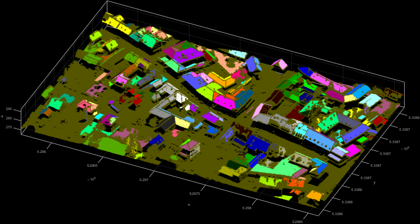
The first example uses an 5° angle difference criterion between adjacent normal vector.
Remark: The constant 0.996 in the above homogenity criterion approximates the cosine of 5°. Figure 2 shows the resulting 3D point cloud coloured by SegmentID.

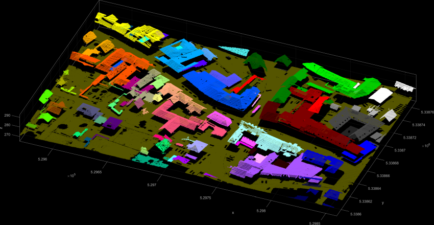
The second example uses the difference in the z-coordinates of neighbouring points as local homogeneity criterion. Neighbouring points belong to the same segment if their difference in the z-component is below 15 cm. The resulting Figure 3 shows spatially connected roofs in the same segment.

The third example uses the railway.laz dataset to show a very basic use of the plane extraction.

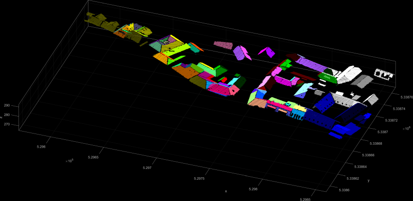
The fourth example shows a more specific use-case for the extraction of planar segments within a given region. Segment seed points have a NormalSigma0 of less than and need to be at a height of Z > 275 m. Thus the resulting segments in Figure 5 show extracted roof faces.

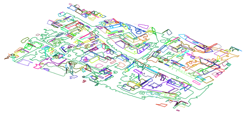
Similar to the previous example roof planes are extracted. But this time also \(\alpha\)-shapes of the segments are computed by defining an alphaRadius of 2m. The alpha shapes are accessible via the segment manager (see example 6) or by creating an additional ODM using the byproduct parameter. The following command line sequence creates strip21_segs.odm which contains the bounding boxes and the \(\alpha\)-shapes of all segments as 3D polylines. To retrieve the \(\alpha\)-shapes as shape file use Module Export with an appropriate filter.

In the examples section it is shown how the segment manager object and segment objects (including their points) can be accessed in C++ (demoSegmentation.cpp) and Python (demoSegmentation.py). These are useful features if further processing of e.g. plane parameters or segment points are desired.

Pöchtrager, M., 2016. Segmentierung Großer Punktwolken Mittels Region Growing. http://katalog.ub.tuwien.ac.at/AC13112627