Module StripAdjust

Table of Contents

• Aim of module
• Requirements for usage of opalsStripAdjust
• General description
  • Strip adjustment workflow
  • Scanner and mounting calibration
  • Trajectory correction parameters
  • Strip adjustment & aerotriangulation
  • Staged processing
  • Distributed / selective processing
  • Internal files
  • Result Files
• Parameter description
• Examples
  • Example 1: Laser scanning strip adjustment
    • Using executable from the command line
    • Using Python module
    • Using C++ interface
    • Processing
  • Example 2: Hybrid laser/image orientation with loose images
  • Example 3: Hybrid laser/image orientation with coupled images
• References

See also

opals::IStripAdjust

Aim of module

Improves the geo-referencing of ALS data and aerial images in a rigorous way combining strip adjustment and aerial triangulation.

Requirements for usage of opalsStripAdjust

This module requires the installation of the Matlab runtime.

General description

Rigorous strip adjustment re-calibrates the ALS multisensor system taking into account original scanner and trajectory measurements. Using the redundancy in the overlapping area of two or more strips, systematic errors in the measurement process are corrected. The impact of these errors can be identified as discrepancies between two overlapping ALS strips or between an ALS strip and a control point cloud. It is furthermore possible to integrate images into the adjustment, i.e. combine ALS strip adjustment and aerial triangulation.

For the determination of discrepancies, a framework similar to Module ICP is adopted. Correspondences are established directly between the point clouds in object space to exploit the full resolution. For the distances, a point-to plane metric is used, i.e. instead of the Euclidean distance between two points its component in the direction of the surface normal is considered.

The decisive difference of rigorous strip adjustment compared to the ICP algorithm is that rather than estimating transformation parameters in object space, correction parameters for the original ALS observations are determined and the direct georeferencing of the point clouds is iteratively improved. That means Module StripAdjust is specialized for ALS data and is not applicable to arbitrary point clouds.

Note that Module StripAdjust strictly uses the degree (full circle=360°) as angular unit in its parameter interface. This applies to values as well as to standard deviations. Alike, angular values are logged, reported, and exported to files in degrees. Following the general rule of OPALS, angles are stored in radians internally, however. Hence, for angles read from file (trajectories and exterior image orientations), the conversion factor to radians must be provided in the respective OPALS Format Definition file (toOpals).

In the following subsection, the basic procedure of Module StripAdjust is outlined. (Glira et al., 2015) provides a more detailed description.

Strip adjustment workflow

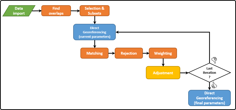
Figure 1: Outline of the StripAdjustment workflow (blue=operations on each ALS strip; orange=operations on all point cloud pairs).

Import of input data: since ALS is a multisensor system, three different types of input data are required (c.f. Module DirectGeoref):

• ALS point clouds in the laser scanner's own coordinate system (SOCS) \(\mathbf{x}^s(t)\).
• Mounting shift and rotation denoted as lever arm \(\mathbf{a}^i\) and boresight misalignment parametrized through three Euler angles \(\mathbf{R}_s^i = \mathbf{R}_s^i(\omega,\phi,\kappa)\). The mounting refers to the INS system and therefore always has the axis directions F-R-D, independent of scanner orientation.
• Trajectory position \(\mathbf{g}^e(t)\) and orientation \(\mathbf{R}_i^n(t) = \mathbf{R}_i^n(\phi(t),\theta(t),\psi(t))\). The three angles correspond to roll ( \(\phi\)), pitch ( \(\theta\)) and yaw ( \(\psi\)) of the aircraft.

Further optional inputs are supported for datum definition or a combined adjustment of ALS and image data:

• Control point clouds as reference data. If no control point clouds are available, the datum of the block can alternatively be defined by fixing the trajectory of one or more strips.
• Image orientations: initial interior orientation and lens distortion parameters for each camera, as well as exterior orientation parameters and a time stamp for each image.
• Image point observations: image points have to be detected using external software and are introduced to Module StripAdjust via text files (c.f. Strip adjustment & aerotriangulation).
• Ground control points: reference object points for aerotriangulation. GCPs are linked to image measurements via corresponding IDs. Other image points merely serve as tie points whose positions are forward intersected into object space.
• Ground tie points: object coordinates of tie points. Just like GCPs, TPs are linked to image measurements via corresponding IDs. If provided, their positions are used unchanged, by-passing their forward intersection.

Direct georeferencing: the ALS point clouds are georeferenced for further processing i.e. the point coordinates in object space are derived from the SOCS coordinates, trajectory and mounting parameters. In the first iteration, the initial values are used. Subsequently, these are (repeatedly) updated in the adjustment step. The relation between a point in the laser scanner's coordinate system ( \(\mathbf{x}^s(t)\)) and the point in a global reference system ( \(\mathbf{x}^e(t)\)) is formulated in the direct georeferencing equation:

\(\mathbf{x}^e(t) = \mathbf{g}^e(t) + \mathbf{R}_n^e(t)\cdot\mathbf{R}_i^n(t)\cdot \Big(\mathbf{a}^i + \mathbf{R}_s^i\cdot\mathbf{x}^s(t) \Big)\)

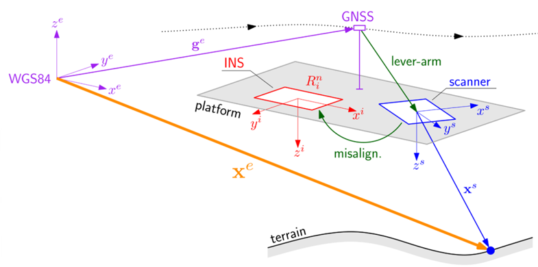
Figure 2: Direct Georeferencing of ALS multisensor data. The scanner observes a point on the ground in its own system, with the platform position determined by the GNSS antenna and its attitude by the INS.

Four different coordinate systems are used here: the scanner coordinate system (s, blue in figure 2), the INS (or "body") coordinate system (i, red), the navigation coordinate system (n, left out in figure 2) and the Earth-Centered, Earth-Fixed (ECEF) coordinate system (e, purple). The rotation matrix from navigation to ECEF system \(\mathbf{R}_n^e(t)\) is not observed but depends on latitude and longitude corresponding to the actual \(\mathbf{g}^e(t)\). Both the establishment of correspondences and the adjustment step are performed in the ECEF system.

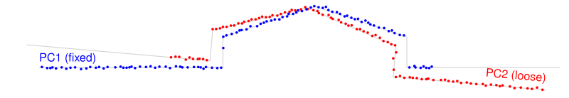
Figure 3: Point cloud pair after direct georeferencing.

Find overlaps: adjustment.voxelSize defines the edge length of a global voxel structure. If the number of voxels that contain points from two different point clouds is higher than the specified threshold (-correspondences.{strip2strip,control2strip,image2strip}.overlap), then these point clouds are considered to overlap. In the most general case, overlaps are checked between three point cloud types:

• ALS strip point clouds
• Control point clouds (if specified)
• Tie points in object space (if image data are specified)

In the following steps, correspondences are established among ALS point clouds and between ALS point clouds and point clouds of a different type.

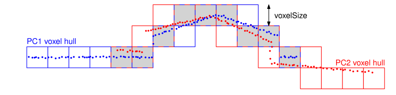
Figure 4: Voxel structure with voxels containing points from different point clouds in grey.

Query point selection & point cloud subsets: Query points are selected for each ALS strip point cloud. The available strategies are the same as in Module ICP and are shortly summarized here (ordered by growing complexity):

• Uniform Sampling (US): Uniform selection of the points in object space based on the voxel structure.
• Normal Space Sampling (NSS): Class-wise sampling in angular space aiming at a uniform distribution of normal vectors (terrain slope & aspect).
• Maximum Leverage Sampling (MLS): Selection of the points with highest leverage providing the strongest constraints for parameter estimation.

Note that in Module StripAdjust the sampling strategies are applied sequentially. First, uniform sampling is used and then the selected query points can be further subselected with NSS or MLS. The optimal strategy depends on the amount and characteristics of ALS data in combination with the computational resources but also on the topography of the scanned objects/landscapes.

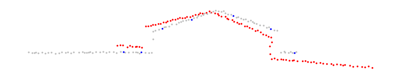
Figure 5: Selection of query points in a point cloud (in this case using uniform sampling).

The selected query points are used to reduce the point clouds for further processing: until their final export, only subsets within a certain radius (-{strips,control}.subsetRadius) around the query points are used instead of the full point clouds. Furthermore, the remaining point clouds can be thinned out to be below the point density specified by -{strips,control}.maxPointDensity, which is recommended for densities above 10 points per square meter. Subsets are created before the first iteration and are not modified during further processing. Therefore, the radius has to be chosen large enough such that establishing correspondences and estimating normals is still possible and meaningful (without extrapolation), even if the point clouds move in object space due to updated parameters (e.g. mounting). On the other hand, a too large subset radius results in higher memory usage than necessary.

For large projects, the recommendation is to use a small subblock (2 strips) with a large subset radius for estimating the mounting parameters and to introduce these parameters as an input for the adjustment of the entire block. Since this minimizes the expected movement of the point clouds, a smaller value for the subset radius can be chosen.

Matching of the potential correspondences. For each query point, its nearest neighbour in each overlapping point cloud is found as correspondence candidate.

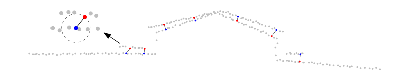
Figure 6: Matching of query points to their closest points in the other point cloud.

Rejection of correspondences: A correspondence is defined as a pair of points (c.f. Matching) that belong to different point clouds, along with their normal vectors.

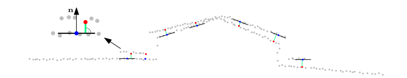
Figure 7: Correspondences and the respective point-to-plane distances (green).

The use of point-to-plane distances (projection of the difference vector onto the normal vector) does not necessitate identical points in object space, but the points have to lie on the same surface. Since this is not the case for all correspondences, potential outliers are eliminated regarding three criteria:

• Plane roughness as a measure of the normal vector reliability.
• Angle between the normal vectors to indicate if the points are on the same plane.
• Distance between the points
• Point-to-plane distance in relation to the a priori assumptions.

Weighting: The remaining correspondences are weighted based on surface roughness and the angle between the respective surface normals.

Least-squares adjustment: point-to-plane distances between corresponding points are minimized by estimating the following parameter groups:

• Scanner calibration parameters (c.f. Scanner and mounting calibration)
• Mounting calibration parameters (c.f. Scanner and mounting calibration)
• Trajectory correction parameters (c.f. Trajectory correction parameters)
• Image exterior and interior orientation parameters including distortions (+ camera mounting, c.f. Strip adjustment & aerotriangulation)

The objective of the adjustment is to minimize the weighted sum of point-to-plane distances.

\(\sum_{i=1}^{\sharp corresp.}(\omega_i \cdot d_i^2) \longrightarrow min\) with \(d_i = (\mathbf{p}_i - \mathbf{q}_i)^T \cdot \mathbf{n}_i\)

The stochastic model is given by the weights \(\omega_i\) and the functional model by the point-to-plane distances \(d_i\); \(\mathbf{p}_i\) and \(\mathbf{q}_i\) are the corresponding points of the \(i\)-th correspondence as determined by the direct georeferencing equation; \(\mathbf{n}_i\) is the unit normal vector in point \(\mathbf{p}_i\).

Until the specified number of iterations is reached, the iteration starts again with direct georeferencing using the updated parameters. Otherwise, the final parameters are used to directly georeference the whole data set, providing adjusted point clouds as output. If images are included in the adjustment, they can optionally be undistorted using the estimated lens distortion parameters. The final interior and exterior image orientations are provided in separate files.

Scanner and mounting calibration

To compensate for systematic errors occuring in the scanner measurement process, scanner calibration parameters are estimated in the adjustment step (on-the-job calibration). Every point \(\mathbf{x}^s\) in the scanner coordinate system is assumed to be the result of one range and two angle measurements i.e. as a function of the three polar coordinates \(\rho\), \(\alpha\) and \(\beta\):

\(\mathbf{x}^s(t) = \rho(t) \cdot \begin{pmatrix} \cos\alpha(t)\sin\beta(t) \\ \sin\alpha(t) \\ \cos\alpha(t)\cos\beta(t) \end{pmatrix}\)

The polar coordinates are determined using the initial values ( \(\rho_0\), \(\alpha_0\), \(\beta_0\)) given by the input data \(\mathbf{x}^s\) and two estimated calibration parameters each:
an offset ( \(\Delta\rho\), \(\Delta\alpha\), \(\Delta\beta\)) and a scale ( \(\epsilon_{\rho}\), \(\epsilon_{\alpha}\), \(\epsilon_{\beta}\)) parameter, making a total of six scanner calibration parameters.

\(\rho(t) = \Delta\rho + \rho_0(t)\cdot(1+\epsilon_{\rho})\)

\(\alpha(t) = \Delta\alpha + \alpha_0(t)\cdot(1+\epsilon_{\alpha})\)

\(\beta(t) = \Delta\beta + \beta_0(t)\cdot(1+\epsilon_{\beta})\)

The mounting calibration parameters describe the rotation from the scanner system to the INS system (misalignment) and the translation between the scanner system and the GNSS antenna (lever arm). In total, six parameters are estimated, namely three misalignment angles ( \(\omega\), \(\phi\), \(\kappa\)) and three lever arm components ( \(a_x\), \(a_y\), \(a_z\)). The axis orientation is F-R-D, independent of scanner orientation. Usually, these parameters are known in advance, but unless they are completely reliable and up-to-date, a re-estimation during the adjustment is reasonable. This particularly concerns the misalignment angles since the impact of a respective error grows with \(\rho\) and thus can become rather large for typical ALS settings.

Trajectory correction parameters

The aircraft trajectory is given by the three element position vector \(\mathbf{g}^e(t) = [g_x^e(t), g_y^e(t), g_z^e(t)]^T\) and three rotation angles roll \(\phi(t)\), pitch \(\theta(t)\) and yaw \(\psi(t)\). The initial values as measured by the GNSS/IMU system are given by \(\mathbf{g}_0^e(t)\) and \(\phi_0(t)\), \(\theta_0(t)\), \(\psi_0(t)\). In contrast to scanner and mounting calibration parameters, where no short-term changes are expected, systematic trajectory errors may vary significantly during short time periods due to different external influences. Therefore, trajectory correction parameters have to be separately estimated for each strip. In case of very unstable trajectory accuracy, time-dependent trajectory correction parameters are necessary. Module StripAdjust offers three different trajectory correction models (listed in order of growing complexity):

Bias trajectory correction model (BTCM): The simplest approach relies on the assumption that the trajectory error does not change significantly within one strip. In this case, an offset ( \(\Delta\phi_j\), \(\Delta\theta_j\), \(\Delta\psi_j\), \(\Delta g_{x,j}^e\), \(\Delta g_{y,j}^e\), \(\Delta g_{z,j}^e\)) for each strip and each of the six trajectory parameters is sufficient:

\(\phi(t) = \phi_0(t) + \Delta\phi_j\)

\(\theta(t) = \theta_0(t) + \Delta\theta_j\)

\(\psi(t) = \psi_0(t) + \Delta\psi_j\)

\(g_x^e(t) = g_{x0}^e(t) + \Delta g_{x,j}^e\)

\(g_y^e(t) = g_{y0}^e(t) + \Delta g_{y,j}^e\)

\(g_z^e(t) = g_{z0}^e(t) + \Delta g_{z,j}^e\)

The index \(j\) stands for the \(j\)-th strip. The total number of parameters is \(6\cdot s\) with \(s\) being the number of strips. For brevity, the following two models are described only by example of \(\phi\), but the descriptions are analogously valid for the other parameters.

Linear trajectory correction model (LTCM): A linear correction model is still rather simple allowing to compensate for parameter offsets and drifts. For each rotation angle, position coordinate, and strip, two correction parameters \(a_0\), \(a_1\) are estimated:

\(\phi(t) = \phi_0(t) + a_{0,j}^{(\phi)} + a_{1,j}^{(\phi)}\cdot(t-t_j^s)\)

where \(t_j^s\) is the start time of strip \(j\). The total number of parameters amounts to \(12\cdot s\).

Spline trajectory correction model (STCM, Glira et al., 2016): For highest flexibility of the trajectory correction, this model works with natural cubic splines. Each strip is divided into segments of equal length \(\Delta t\) and for each segment, the time-dependent correction is estimated as a cubic polynomial. For the \(k\)-th segment of the \(j\)-th strip the time dependent correction of the roll angle \(\phi\) has the form

\(\Delta\phi_{j,k}(t) = a_{0,j,k}^{(\phi)} + a_{1,j,k}^{(\phi)}\cdot(t-t_{j,k}^s) + a_{2,j,k}^{(\phi)}\cdot(t-t_{j,k}^s)^2 + a_{3,j,k}^{(\phi)}\cdot(t-t_{j,k}^s)^3\)

where \(t_{j,k}^s\) is the start time of the segment. For each segment, four parameters \(a_{0,j,k}\) to \(a_{3,j,k}\) are estimated. The total number of parameters depends on the number of strips \(s\) and on the number of segments of each strip \(n_j\) (factor 6 considers the three rotation angles and position vector components): \(6\cdot4\cdot \sum_{j=1}^{s}n_j\).

To ensure a continuous and smooth correction function throughout a whole strip, additional constraints are introduced for each junction requiring continuity of the function value as well as its first and second derivatives. Furthermore, the first and second derivatives can be optionally set to zero at the beginning and at the end of each strip.

Short segment lenghts \(\Delta t\) allow for a great flexibility of the correction function and pose the risk of overfitting and respective block deformations. Hence, they require a dense and homogeneous distribution of correspondences to estimate the resulting high number of parameters with sufficient redundancy. Also, it its recommended to use control point clouds if STCM is applied.

After the last iteration the corrected trajectory is exported stripwise in two different versions. The trajectories saved in strip_traj_ins refer to the INS (body) coordinate system. For the trajectories in strip_traj_scanner, the lever arm and misalignment have additionally been applied, i.e. the respective position and orientation describe the scanner system.

Strip adjustment & aerotriangulation

As already outlined in the general description, it is possible to perform a hybrid adjustment of ALS and photogrammetric data, combining ALS strip adjustment with bundle block adjustment. Like in ALS strip adjustment, point-to-plane distances between all respective point clouds in object space are then minimized. Furthermore, ground control points (GCP) for the images can be introduced. These are given by their 3D coordinates in UTM along with an id (attribute _pointID) linking them to image measurements (c.f. observation text file).

While exterior image orientations are independent of the flight trajectory (loose) by default, they may alternatively be coupled to it. Just like scanners, cameras then relate to the body coordinate system by a resp. mounting calibration consisting of a lever arm and a misalignment. The assignment of a strip index to images.images.strip ties an image to that strip's trajectory. Unlike in an uncoupled, hybrid adjustment, time stamps are needed for each image, which are used to interpolate from the flight trajectory the position and attitude of the body coordinate system at the time of exposure. Unless tie point object coordinates are given (groundTiePoints.inFile), they are computed by an initial forward intersection. This requires good enough estimates of the camera mounting calibration parameters (lever arm and misalignment angles). If not set, these are automatically estimated, if exterior image orientations are provided in addition to time stamps.

The following parameter types related to the image data can be estimated:

• Interior orientation: corrections for the interior orientation parameters ( \(c\), \(x_0\), \(y_0\)) for each camera. Furthermore, two radial ( \(a_3\), \(a_4\)) and two tangential ( \(a_5\), \(a_6\)) lens distortion parameters. If it is unsure whether these parameters can compensate the given image distortions, it is recommended to undistort the images beforehand using external software.
• Object point coordinates: the adjusted tie and ground control points in object space are provided as SHP files.
• Loose images:
  • Exterior image orientation parameters (images.images.extOri)
• Coupled images:
  • Camera mounting: like for Laser scanners, lever arm (cameras.leverArm) and misalignment (cameras.misalignment) can be estimated for each camera w.r.t. the trajectory.
  • Exterior image orientation corrections (images.images.dExtOri): corrections to the exterior image orientations derived from the trajectory for each image separately.

For details on camera and image parameters, see Photogrammetric Conventions .

Image timestamps and / or a priori exterior orientations must be given in a file (images.images.oriFile) whose structure is to be specified by an according OFD file (images.images.oriFormat), with timestamp entries as GPSTime, and exterior orientations as X0, Y0, Z0, OmegaAngle, PhiAngle, and KappaAngle, with angles in radians. Since several images may share the same timestamp / EOR file, each image needs to be matched with a single file record. This is done via the entry PointLabel, which needs to be identical to the respective image file name.

Due to their high number, image point observations are expected in a separate text file for each image (images.images.obsFile). Such a text file must provide the point id and image coordinates (x,y) of all points observed in the respective image:

1007 3891.270 -154.134
1009 3245.010 -58.492 
1013 3230.410 -58.381 
1018 3245.010 -58.492 
1019 4023.310 -130.005
1036 3744.890 -158.324
1038 3266.350 -191.740
1041 3861.700 -133.732
2421 3162.320 -158.465
2424 4224.560 -61.815 
[...]

Potentially included further columns in this file (e.g. quality measures) will be ignored.

Staged processing

The workflow of Module StripAdjust is organized as a sequence of stages:

• importData : import all data into internal, temporary files.
• preprocess : forward intersect image points, determine overlapping point clouds, select query points, create point cloud subsets.
• adjust : loop over direct georeferencing, matching, rejection and weighting of correspondences, and adjustment.
• postprocess : forward intersect image points with final parameters.
• exportData : export everything but the strip data (e.g. correspondences, corrected trajectory).
• exportStrips : export the ALS strip data, directly georeferenced using the adjusted parameters.

Using workflow.stages.first and workflow.stages.last, an inclusive range of these stages can be selected for processing. Having set workflow.stages.first to anything but importData, Module StripAdjust restores intermediate results, and it overwrites the parameters of the current call with those that these results are based on, except for parameters in the group workflow.

Hence, processing may e.g. be stopped after the adjustment stage to inspect the log, and be resumed afterwards. To achieve this, call Module StripAdjust once with workflow.stages.last set to adjust, and another time with workflow.stages.first set to postprocess and otherwise unchanged parameters. Note that if workflow.stages.first and workflow.stages.last cover the whole range of stages, Module StripAdjust deletes its intermediate results by default, making it impossible for a subsequent call to resume processing (see tempData.cleanup).

For executing exportStrips only, the parameters affecting the import and export of each strip may be changed in addition to the parameters in the group workflow: strips.strips.inFile, strips.strips.iFormat, strips.strips.filter.gridMask, strips.strips.filter.iFilter, strips.strips.outFile, and strips.strips.oFormat. Hence, it is e.g. possible to execute the adjustment with thinned out ALS data, and then apply the adjusted parameters to the original ALS data by subsequently calling Module StripAdjust with workflow.stages.first set to exportStrips and accordingly different ALS strip file paths (strips.strips.inFile). Apart from the possibly different import / export parameters, the same parameters still apply for the strip at the respective index, particularly the session ID and trajectory parameters. Furthermore, the total number of strips must not be changed, and only those points of each replacement strip file get exported whose timestamps are included in the range of timestamps of the strip file used for the adjustment.

Distributed / selective processing

Some stages can be told to process only a subset of all data by setting workflow.strips, workflow.controlPointClouds, and workflow.images:

• importData
• exportData
• exportStrips

These stages must then be processed separately from the preceeding and succeeding stages that are not in this list.

Using this feature and Staged processing, the workload of importing and/or exporting data may be distributed over separate machines that may do their tasks concurrently. As a precondition, Module StripAdjust must be called with the same parameters on all machines (with the exceptions mentioned above) and an outDirectory that points to the same network folder.

Internal files

The core functionality of Module StripAdjust is implemented in MATLAB. Internal .mat files are stored in the outDirectory and tempData.directory folders. The following table lists the internal files and folders together with a short content description and the processing phase in which the corresponding data are generated. Note that files in tempData.directory remaining from a previous program run may be reused in a later run.

File/Folder	Description	Generation phase
outDirectory/p.mat	Internal project file
outDirectory/stripAdjustmentResults.mat	Internal result file
tempData.directory/STRRAW	For each strip a .mat file with the corresponding strip file name exists containing all laser points (before applying strips.strips.filter.iFilter). Each point consists of the sensor coordinates (converted to F-R-D), all attributes, an internal ID, the time-interpolated trajectory data (i.e. X, Y, Z, roll, pitch, yaw), and additional meta data like center-of-gravity, number of points, bounding box, etc. The additional _info.mat file contains the time range covered by the strip (t_min, t_max).	importData
tempData.directory/STR	For each strip a .mat file with the corresponding strip file name exists containing the filtered (strips.strips.filter.iFilter), directly georeferenced points (ECEF). Beyond that, the same attributes and meta data as above for STRRAW are provided.	importData
tempData.directory/STRVH	For each strip a .mat file with the corresponding strip file name exists containing the voxel hull in ECEF coordinates. Each point represents the center of a voxel containing laser points.	importData
tempData.directory/STR2STR	File pairs.mat contains a list of overlapping strip pairs (indices of overlapping strips and respective statistics).	preprocess
tempData.directory/CPC2STR	File pairs.mat contains a list of overlapping control point clouds and strips (pairs of CPC id / strip id, respective statistics).	preprocess
tempData.directory/IMG2STR	File pairs.mat contains a list of overlapping image tie points and strips (strip id, respective statistics).	preprocess
tempData.directory/CP	The folder contains the sub-folders STR2STR, CPC2STR, and IMG2STR. In each of these sub-folders the file queryPoints.mat contains a table of query points (in ECEF) for each overlapping pair.	preprocess
tempData.directory/STRRAWSUB	For each strip a .mat file with the corresponding strip file name exists containing all points of the STRRAW dataset reduced to the subset area.	preprocess
tempData.directory/STRSUB	For each strip a .mat file with the corresponding strip file name exists containing the directly georeferenced points of STRRAWSUB. All data in STRSUB are re-caculated in the individual iterations (phase: adjust) using the current parameters (lever arm, boresight angles, trajectory corrections, etc.).	adjust

Result Files

Module StripAdjust generates report and different result files in the output folder (outDirectory). The following table provides a detailed description of the provided datasets.

File/Folder	Description
stripAdjustmentReport_JJJJMMDD_HHMMSS.XXX.txt	Report file of a single Module StripAdjust run (text)
correspondences	The folder contains the sub-folders STR2STR, CPC2STR, and IMG2STR. Each sub-folder contains a separate (.shp) file for each overlapping dataset pair (laser strips, control point clouds and strips, image tie points and strips) containing the locations of correspondences in UTM coordinates.
images/tie_points	The folder contains the 3D image tie points in UTM coordinates (easting, northing, ellipsoidal height, point id) in shp and xyz text file format (image_tie_points.*). Files image_tie_points_tripost.* contain the 3D tie points resulting from image ray forward intersection using the IORs and EORs estimated within the hybrid adjustment to be used for post-adjustment quality control.
images/distorted_images	The folder contains the estimated EORs and IORs of the original images in UTM (image_orientations.*) and ECEF (image_orientations_ecef.*), both in shp and xyz text format.
images/undistorted_images	The folder contains the estimated EORs and IORs of the disortion-free images in UTM (image_orientations.*) and ECEF (image_orientations_ecef.*), both in shp and xyz text format. In addition to the image orientations, the folder also contains the undistorted images.
strips	The folder contains the calibrated/oriented strips in UTM coordinates.
trajectories	The folder contains the sub-folders ins and scanner. Each sub-folder contains the flight strip trajectories (UTM easting, UTM northing, ellipsoidal height, time, roll, pitch, yaw) in corresponding files with reference to the INS or scanner coordinate system, respectively.

Parameter description

-outDirectoryOutput directory

Type: opals::Path
Remarks: default=stripAdjust
Store the final processing results within this folder.

-oFilterOutput filter

Type: opals::Filter<DM::IFilter::ReadAccess::coordinatesAttributes, DM::IFilter::WriteAccess::coordinates | attributes | delayedResults>
Remarks: optional
Save only those strip points to file that pass this filter.
Filter<coordinatesAttributes, coordinates | attributes | delayedResults>: has read access to: coordinatesAttributes; has write access to: coordinates | attributes | delayedResults;
See Filters

-tempDataIGroup: Options concerning temporary / intermediate data storage

.directoryRoot directory of all temporary data

Type: opals::Path
Remarks: estimable
All intermediate data is stored within this directory, preferably on a fast drive. Estimation rule: <outDirectory>/temp.

.cleanupDelete temporary data

Type: bool
Remarks: mandatory
If true, delete this directory at the beginning and end of the run. If unset, assume yes if all workflow stages are to be processed.

.compressCompress intermediate data

Type: bool
Remarks: default=1
Compress temporary data. Results in less temporary storage space used, but considerably slows down file access on fast drives like local SSDs.

-utmIGroup: UTM information for the projection of data in ECEF system

.zoneUTM zone

Type: uint32
Remarks: mandatory
Zone numbers range from 1 to 60; the zone depends on the longitude of the project area

.hemisphereUTM hemisphere

Type: opals::Hemisphere
Remarks: mandatory

Possible values:  
  north ... Northern hemisphere
  south ... Southern hemisphere

Choose the hemisphere within the UTM zone

-adjustmentIGroup: Adjustment options

.voxelSizeVoxel size

Type: double
Remarks: default=10
The edge length of each voxel used to find overlaps between point clouds in object space. 100 must be a whole multiple of it: fmod(100,x) == 0.

.maxIterMaximum number of iterations

Type: uint32
Remarks: default=5
The number of iterations through the Strip Adjustment workflow.

.robustIterNumber of robust iterations

Type: uint32
Remarks: default=0

.covarianceCo-variances a posteriori

Type: bool
Remarks: default=0
Estimate and assign standard deviations of parameters a posteriori, and log their highest correlations.

-stripsIGroup: Options concerning all ALS strips.

.stripsIVector: Options concerning the input ALS strips

Please note that strip indices are shifted by 1 from the input to the log output, i.e. strips[0] will in the output be adressed as strip 1.

.allIGroup: default element

.inFileInput files

Type: opals::Path
Remarks: mandatory
The ALS strips are expected as separate files.The points have to be in the scanner's coordinate system with GPSTime.

.iFormatinput file format [auto, sdc, <opals format def. xml file>, ...]

Type: opals::String
Remarks: default=auto
Explicitly specify the input file format.
Estimation rule: auto: the file content is used to recognise the file format.

.outFileoutput directory or file path

Type: opals::Path
Remarks: mandatory
Explicitly specify the output directory or file path. If given path ends in a directory separator, it is considered a directory. In that case, the file name is adopted from input.
Estimation rule: <outDirectory>/strips/<inFile-basename>.<oFormat-extension>

.calcScanAnglecompute the attribute ScanAngle

Type: bool
Remarks: default=1
Compute the attribute ScanAngle based on the adjusted parameters, and following its definition in the LAS file format standard. Deactivate its computation for speed-up.

.oFormatoutput file format [auto, sdw, las, <opals format def. xml file>, ...]

Type: opals::String
Remarks: default=auto
Explicitly specify the output file format.
Estimation rule: auto: In general, the same format will be used for input and output. For formats not allowing to store potentially large project coordinates with sufficient precision, a suitable substitute is used instead (e.g., sdc->sdw).

.scannerOrientationScanner orientation

Type: opals::ScannerOrientation
Remarks: mandatory

Possible values:  
  frd ... front/right/down
  fdl ... front/down/left
  flu ... front/left/up
  fur ... front/up/right
  bdr ... back/down/right
  bld ... back/left/down
  bul ... back/up/left
  bru ... back/right/up
  lfd ... left/front/down
  ldb ... left/down/back
  lbu ... left/back/up
  luf ... left/up/front
  rdf ... right/down/front
  rbd ... right/back/down
  rub ... right/up/back
  rfu ... right/front/up
  ufl ... up/front/left
  ulb ... up/left/back
  ubr ... up/back/right
  urf ... up/right/front
  dlf ... down/left/front
  dbl ... down/back/left
  drb ... down/right/back
  dfr ... down/front/right

The approximate mounting of the scanner on the platform.

.sessionSession ID

Type: uint32
Remarks: default=0
ALS strips can be assigned to different sessions. A typical application would be the processing of data from multiple acquisition epochs. Scanner and mounting calibration parameters are estimated separately for each session. Note that indexing starts at 0. For setting e.g. the trajectory of the strips assigned to the first session, use -sessions[0].trajectory.inFile .

.filterIGroup: Point cloud filtering

Restricts the points for which correspondences may be established. Irrespective of the filter, all points are considered in the final georeferencing step.

.gridMaskGrid mask file

Type: opals::Path
Remarks: optional
A grid mask can be used to exclude areas that are unsuitable for establishing correspondences, e.g. unstable terrain or water bodies. Only points that fall into pixels with value 1 will be candidates for correspondences.

.iFilterInput filter

Type: opals::Filter<DM::IFilter::ReadAccess::coordinatesAttributes, DM::IFilter::WriteAccess::coordinates | attributes>
Remarks: default=Echo[Last]
See the syntax described in the manual, chapter 'Filters'.
Filter<coordinatesAttributes, coordinates | attributes>: has read access to: coordinatesAttributes; has write access to: coordinates | attributes;
See Filters

.trajectoryIGroup: Options for trajectory correction

.correctionModelTrajectory correction model

Type: opals::TrajectoryCorrectionModel
Remarks: default=linear

Possible values:  
  bias ..... Offsets of position and rotation. Polynomial degree: 0
  linear ... Offsets and scales of position and rotation. Polynomial degree: 1
  spline ... Cubic spline. Polynomial degree: 3

This parameter defines the model used for trajectory correction (c.f. section 'Trajectory correction parameters').

.samplingIntervalTime sampling interval [s]

Type: double
Remarks: default=10
This parameter defines the length of the time segments for which separate trajectory correction functions are estimated. The value of this parameter is only considered in case that a spline trajectory correction model is used. In case of a bias or linear correction model, strips are not split into segments, and the sampling interval length is ignored.

.boundaryDerivativeIsZeroIGroup: zero derivatives on the segment boundary

In order to ensure a flat spline correction function, first and/or second derivative can be set to zero on the boundary between two segments.

.firstSet first derivative zero

Type: bool
Remarks: default=0

.secondSet second derivative zero

Type: bool
Remarks: default=0

.dXIGroup: dX

Trajectory offset X

.valueinitial / adjusted value

Type: double
Remarks: default=0

.sigmaAprioriStandard deviation of direct observation.

Type: double
Remarks: default=-1
If > 0, introduce a direct observation with sigmaApriori as standard deviation a priori. If 0, treat value as constant. If < 0, estimate value without a direct observation.

.dYIGroup: dY

Trajectory offset Y

.valueinitial / adjusted value

Type: double
Remarks: default=0

.sigmaAprioriStandard deviation of direct observation.

Type: double
Remarks: default=-1
If > 0, introduce a direct observation with sigmaApriori as standard deviation a priori. If 0, treat value as constant. If < 0, estimate value without a direct observation.

.dZIGroup: dZ

Trajectory offset Z

.valueinitial / adjusted value

Type: double
Remarks: default=0

.sigmaAprioriStandard deviation of direct observation.

Type: double
Remarks: default=-1
If > 0, introduce a direct observation with sigmaApriori as standard deviation a priori. If 0, treat value as constant. If < 0, estimate value without a direct observation.

.dRollIGroup: dRoll [deg]

Offset of the roll-angle

.valueinitial / adjusted value

Type: double
Remarks: default=0

.sigmaAprioriStandard deviation of direct observation.

Type: double
Remarks: default=-1
If > 0, introduce a direct observation with sigmaApriori as standard deviation a priori. If 0, treat value as constant. If < 0, estimate value without a direct observation.

.dPitchIGroup: dPitch [deg]

Offset of the pitch-angle

.valueinitial / adjusted value

Type: double
Remarks: default=0

.sigmaAprioriStandard deviation of direct observation.

Type: double
Remarks: default=-1
If > 0, introduce a direct observation with sigmaApriori as standard deviation a priori. If 0, treat value as constant. If < 0, estimate value without a direct observation.

.dYawIGroup: dYaw [deg]

Offset of the yaw-angle

.valueinitial / adjusted value

Type: double
Remarks: default=0

.sigmaAprioriStandard deviation of direct observation.

Type: double
Remarks: default=-1
If > 0, introduce a direct observation with sigmaApriori as standard deviation a priori. If 0, treat value as constant. If < 0, estimate value without a direct observation.

.normalsIGroup: Options for normal estimation

These parameters are generally used to compute normal vectors for strip point clouds. However, when computing normals to match a strip with control point clouds, controlPointClouds.normals is used both for the strip and the control point clouds.

.searchRadiusSearch radius for plane fitting

Type: double
Remarks: default=2
For estimating the normal vector in one point, all neighbouring points within the search radius are used to fit a plane. The resulting normal vector is necessary for calculating point-to-plane distances. Additionally it is used (along with the roughness value) for rejection of false correspondences.

.neighboursMinimum number of neighbours for normal estimation

Type: uint32
Remarks: default=8
Lower limit for the number of neighbours to result in a reliable plane fit.

.subsetRadiusRadius of subset areas

Type: double
Remarks: estimable
Selecting subsets is necessary for many ALS flight blocks since typically, the full amount of data can't be loaded into memory simultaneously. Therefore, only smaller subsets around the correspondences are loaded (c.f. 'Correspondence Selection & Subsets' in the Workflow description). If positive, use as radius for subset selection. If negative, use an infinite radius i.e. use all data as subsets. Estimation rule: 2 * normals.searchRadius

.maxPointDensityMaximum point density

Type: double
Remarks: optional
Unit: [points per square unit length (e.g. meter)]. Limiting the point density can for example be useful in case of UAV-borne laserscanning where possibly tremendous point densities occur.

-controlPointCloudsIGroup: Control point clouds

Introduces ground-truth data in the form of general point clouds in UTM system. These point clouds can for example be the result of terrestrial laser scanning or former ALS campaigns but also vectorized height models etc.

.inFilePaths to optional control point clouds

Type: opals::Vector<opals::Path>
Remarks: default=
Note that wildcard characters (*,?) can be used for the selection of multiple files at once (e.g. controlPointClouds/cpc*.xyz)

.iFormatfile format [auto, odm, las, <opals format def. xml file>, ...]

Type: opals::Vector<opals::String>
Remarks: default=auto
Explicitly specify the file format - either 1 format for all files, or 1 for each of them.
Estimation rule: auto: the file content is used to recognise the file format.

.normalsIGroup: Normal calculation for control point clouds

As for the ALS strips, normals also have to be estimated for the control point clouds. Due to the possibly different point density, separate parameters are defined. For a more detailed description please refer to the respective parameters for ALS normal estimation above.

.searchRadiusSearch radius for plane fitting

Type: double
Remarks: default=3

.neighboursMinimum number of neighbours for normal estimation

Type: uint32
Remarks: default=5

.subsetRadiusControl point cloud subset radius

Type: double
Remarks: default=-1
If positive, use as radius for subset selection. If negative, use an infinite radius i.e. use all data as subsets.

.maxPointDensityMaximum point density of control point clouds

Type: double
Remarks: optional
Unit: [points per square unit length (e.g. meter)].

-groundControlPointsIGroup: Ground control points

Control and check points for image point observations, identified by their ID.

.inFileInput file path

Type: opals::Path
Remarks: optional
File must contain X, Y, Z in UTM, and _pointId as point ID

.iFormatfile format [auto, odm, las, <opals format def. xml file>, ...]

Type: opals::String
Remarks: default=auto
Explicitly specify the file format.
Estimation rule: auto: the file content is used to recognise the file format.

.XIGroup: X

.sigmaAprioriStandard deviation of ground control points X coordinates.

Type: double
Remarks: default=0.005
Introduce a direct observation of the X coordinate with sigmaApriori as standard deviation a priori (ECEF).

.YIGroup: Y

.sigmaAprioriStandard deviation of ground control points Y coordinates.

Type: double
Remarks: default=0.005
Introduce a direct observation of the Y coordinate with sigmaApriori as standard deviation a priori (ECEF).

.ZIGroup: Z

.sigmaAprioriStandard deviation of ground control points Z coordinates.

Type: double
Remarks: default=0.005
Introduce a direct observation of the Z coordinate with sigmaApriori as standard deviation a priori (ECEF).

.checkPointsCheck point IDs

Type: opals::Vector<int32>
Remarks: default=
Do not introduce these points into the adjustment.

-groundTiePointsIGroup: Tie point object coordinates

Object coordinates of tie points for image point observations, identified by their ID. If provided, then forward intersection is skipped

.inFileInput file path

Type: opals::Path
Remarks: optional
File must contain X, Y, Z in UTM, and _pointId as point ID

.iFormatfile format [auto, odm, las, <opals format def. xml file>, ...]

Type: opals::String
Remarks: default=auto
Explicitly specify the file format.
Estimation rule: auto: the file content is used to recognise the file format.

-imagesIGroup: Options concerning image data

.imagesIVector: Options concerning the input images

Please note that indices are shifted by 1 from the input to the log output, i.e. images[0] will in the output be adressed as image 1.

.allIGroup: default element

.inFileInput image files

Type: opals::Path
Remarks: mandatory
Image files are used for optional undistortion. Tie points have to be measured in advance using external software (c.f. obsFile).

.cameracamera index

Type: uint32
Remarks: default=0
Analogous to sessions, interior orientations are estimated camera-wise. With this parameter, images can be assigned to different cameras.

.stripIndex of corresponding strip

Type: uint32
Remarks: optional
Tie this image to the trajectory of the given strip. If unset, compute an independent image exterior orientation.

.extOriIGroup: Exterior orientation parameters

Values are output only. Standard deviations are irrelevant if image is tied to a strip.

.X0IGroup: X0

.valueadjusted value

Type: double
Remarks: default=-1

.sigmaAprioriStandard deviation of direct observation.

Type: double
Remarks: default=-1
If > 0, introduce a direct observation with sigmaApriori as standard deviation a priori. If 0, treat value as constant. If < 0, estimate value without a direct observation.

.Y0IGroup: Y0

.valueadjusted value

Type: double
Remarks: default=-1

.sigmaAprioriStandard deviation of direct observation.

Type: double
Remarks: default=-1
If > 0, introduce a direct observation with sigmaApriori as standard deviation a priori. If 0, treat value as constant. If < 0, estimate value without a direct observation.

.Z0IGroup: Z0

.valueadjusted value

Type: double
Remarks: default=-1

.sigmaAprioriStandard deviation of direct observation.

Type: double
Remarks: default=-1
If > 0, introduce a direct observation with sigmaApriori as standard deviation a priori. If 0, treat value as constant. If < 0, estimate value without a direct observation.

.omegaIGroup: omega [deg]

.valueadjusted value

Type: double
Remarks: default=-1

.sigmaAprioriStandard deviation of direct observation.

Type: double
Remarks: default=-1
If > 0, introduce a direct observation with sigmaApriori as standard deviation a priori. If 0, treat value as constant. If < 0, estimate value without a direct observation.

.phiIGroup: phi [deg]

.valueadjusted value

Type: double
Remarks: default=-1

.sigmaAprioriStandard deviation of direct observation.

Type: double
Remarks: default=-1
If > 0, introduce a direct observation with sigmaApriori as standard deviation a priori. If 0, treat value as constant. If < 0, estimate value without a direct observation.

.kappaIGroup: kappa [deg]

.valueadjusted value

Type: double
Remarks: default=-1

.sigmaAprioriStandard deviation of direct observation.

Type: double
Remarks: default=-1
If > 0, introduce a direct observation with sigmaApriori as standard deviation a priori. If 0, treat value as constant. If < 0, estimate value without a direct observation.

.dExtOriIGroup: Delta exterior orientation parameters

Only relevant if image is tied to a strip. Values are differences between the actual exterior image orientation and the one derived from the image timestamp, its trajectory, and the camera lever arm and misalignment.

.dX0IGroup: dX0

.valueinitial / adjusted value

Type: double
Remarks: default=0

.sigmaAprioriStandard deviation of direct observation.

Type: double
Remarks: default=0.1
If > 0, introduce a direct observation with sigmaApriori as standard deviation a priori. If 0, treat value as constant. If < 0, estimate value without a direct observation.

.dY0IGroup: dY0

.valueinitial / adjusted value

Type: double
Remarks: default=0

.sigmaAprioriStandard deviation of direct observation.

Type: double
Remarks: default=0.1
If > 0, introduce a direct observation with sigmaApriori as standard deviation a priori. If 0, treat value as constant. If < 0, estimate value without a direct observation.

.dZ0IGroup: dZ0

.valueinitial / adjusted value

Type: double
Remarks: default=0

.sigmaAprioriStandard deviation of direct observation.

Type: double
Remarks: default=0.1
If > 0, introduce a direct observation with sigmaApriori as standard deviation a priori. If 0, treat value as constant. If < 0, estimate value without a direct observation.

.dOmegaIGroup: dOmega [deg]

.valueinitial / adjusted value

Type: double
Remarks: default=0

.sigmaAprioriStandard deviation of direct observation.

Type: double
Remarks: default=0.01
If > 0, introduce a direct observation with sigmaApriori as standard deviation a priori. If 0, treat value as constant. If < 0, estimate value without a direct observation.

.dPhiIGroup: dPhi [deg]

.valueinitial / adjusted value

Type: double
Remarks: default=0

.sigmaAprioriStandard deviation of direct observation.

Type: double
Remarks: default=0.01
If > 0, introduce a direct observation with sigmaApriori as standard deviation a priori. If 0, treat value as constant. If < 0, estimate value without a direct observation.

.dKappaIGroup: dKappa [deg]

.valueinitial / adjusted value

Type: double
Remarks: default=0

.sigmaAprioriStandard deviation of direct observation.

Type: double
Remarks: default=0.01
If > 0, introduce a direct observation with sigmaApriori as standard deviation a priori. If 0, treat value as constant. If < 0, estimate value without a direct observation.

.oriFileTimestamp and / or a priori exterior image orientation (c.f. Section 'Strip adjustment & Aerotriangulation')

Type: opals::Path
Remarks: mandatory
If image is tied to a strip, then this file must contain the image's timestamp [GPSTime].
Otherwise, initial values for exterior image orientation parameters [X0 Y0 Z0 OmegaAngle PhiAngle KappaAngle].
If both are given and the camera mouting calibration is unset, then it is derived from them.
In any case, a PointLabel must be specified for each record in this file, and one of them must match this image's file name.
Angles are expected in radians.

.oriFormatTimestamp / exterior image orientation file format

Type: opals::Path
Remarks: default=ImageTimestampAndOrientation.xml
File format of oriFile as OFD

.obsFileImage point observations (c.f. Section 'Strip adjustment & Aerotriangulation')

Type: opals::Path
Remarks: mandatory
Image coordinates of tie point observations in the current image as provided by external software. Each line contains at least three columns with [tiePointID imgCoordX imgCoordY] separated by whitespace. Further columns are ignored.

.undistortExport undistorted images

Type: bool
Remarks: default=0
If this parameter is set to true, the original images are undistorted using the estimated distortion parameters.

.forwardIntersectIGroup: Forward intersection of tie points

In order to establish correspondences to ALS data, the image tie points are forward intersected to object space.

.extOriIGroup: Exterior orientation parameter standard deviations

Only the standard deviations can be set here, the respective initial values are read from the orientation File (c.f. oriFile)

.X0IGroup: X0

.sigmaAprioriStandard deviation of direct observation.

Type: double
Remarks: default=0.1
If > 0, introduce a direct observation with sigmaApriori as standard deviation a priori. If 0, treat value as constant. If < 0, estimate value without a direct observation.

.Y0IGroup: Y0

.sigmaAprioriStandard deviation of direct observation.

Type: double
Remarks: default=0.1
If > 0, introduce a direct observation with sigmaApriori as standard deviation a priori. If 0, treat value as constant. If < 0, estimate value without a direct observation.

.Z0IGroup: Z0

.sigmaAprioriStandard deviation of direct observation.

Type: double
Remarks: default=0.1
If > 0, introduce a direct observation with sigmaApriori as standard deviation a priori. If 0, treat value as constant. If < 0, estimate value without a direct observation.

.omegaIGroup: omega [deg]

.sigmaAprioriStandard deviation of direct observation.

Type: double
Remarks: default=-1
If > 0, introduce a direct observation with sigmaApriori as standard deviation a priori. If 0, treat value as constant. If < 0, estimate value without a direct observation.

.phiIGroup: phi [deg]

.sigmaAprioriStandard deviation of direct observation.

Type: double
Remarks: default=-1
If > 0, introduce a direct observation with sigmaApriori as standard deviation a priori. If 0, treat value as constant. If < 0, estimate value without a direct observation.

.kappaIGroup: kappa [deg]

.sigmaAprioriStandard deviation of direct observation.

Type: double
Remarks: default=-1
If > 0, introduce a direct observation with sigmaApriori as standard deviation a priori. If 0, treat value as constant. If < 0, estimate value without a direct observation.

.dExtOriIGroup: Delta exterior orientation parameter standard deviations

The respective values are defined in the orientation File (c.f. oriFile)

.dX0IGroup: dX0

.sigmaAprioriStandard deviation of direct observation.

Type: double
Remarks: estimable
If > 0, introduce a direct observation with sigmaApriori as standard deviation a priori. If 0, treat value as constant. If < 0, estimate value without a direct observation.
Estimation rule: use images.images.all.dExtOri.dX0.sigmaApriori

.dY0IGroup: dY0

.sigmaAprioriStandard deviation of direct observation.

Type: double
Remarks: estimable
If > 0, introduce a direct observation with sigmaApriori as standard deviation a priori. If 0, treat value as constant. If < 0, estimate value without a direct observation.
Estimation rule: use images.images.all.dExtOri.dY0.sigmaApriori

.dZ0IGroup: dZ0

.sigmaAprioriStandard deviation of direct observation.

Type: double
Remarks: estimable
If > 0, introduce a direct observation with sigmaApriori as standard deviation a priori. If 0, treat value as constant. If < 0, estimate value without a direct observation.
Estimation rule: use images.images.all.dExtOri.dZ0.sigmaApriori

.dOmegaIGroup: dOmega [deg]

.sigmaAprioriStandard deviation of direct observation.

Type: double
Remarks: estimable
If > 0, introduce a direct observation with sigmaApriori as standard deviation a priori. If 0, treat value as constant. If < 0, estimate value without a direct observation.
Estimation rule: use images.images.all.dExtOri.dOmega.sigmaApriori

.dPhiIGroup: dPhi [deg]

.sigmaAprioriStandard deviation of direct observation.

Type: double
Remarks: estimable
If > 0, introduce a direct observation with sigmaApriori as standard deviation a priori. If 0, treat value as constant. If < 0, estimate value without a direct observation.
Estimation rule: use images.images.all.dExtOri.dPhi.sigmaApriori

.dKappaIGroup: dKappa [deg]

.sigmaAprioriStandard deviation of direct observation.

Type: double
Remarks: estimable
If > 0, introduce a direct observation with sigmaApriori as standard deviation a priori. If 0, treat value as constant. If < 0, estimate value without a direct observation.
Estimation rule: use images.images.all.dExtOri.dKappa.sigmaApriori

.intOriIGroup: Interior orientation parameter standard deviations

.cIGroup: c [px]

.sigmaAprioriStandard deviation of direct observation.

Type: double
Remarks: default=-1
If > 0, introduce a direct observation with sigmaApriori as standard deviation a priori. If 0, treat value as constant. If < 0, estimate value without a direct observation.

.X0IGroup: x0 [px]

.sigmaAprioriStandard deviation of direct observation.

Type: double
Remarks: default=-1
If > 0, introduce a direct observation with sigmaApriori as standard deviation a priori. If 0, treat value as constant. If < 0, estimate value without a direct observation.

.Y0IGroup: y0 [px]

.sigmaAprioriStandard deviation of direct observation.

Type: double
Remarks: default=-1
If > 0, introduce a direct observation with sigmaApriori as standard deviation a priori. If 0, treat value as constant. If < 0, estimate value without a direct observation.

.distortionIGroup: Lens distortion parameter standard deviations

.a3IGroup: a3

Radial distortion 3rd degree

.sigmaAprioriStandard deviation of direct observation.

Type: double
Remarks: default=-1
If > 0, introduce a direct observation with sigmaApriori as standard deviation a priori. If 0, treat value as constant. If < 0, estimate value without a direct observation.

.a4IGroup: a4

Radial distortion 5th degree

.sigmaAprioriStandard deviation of direct observation.

Type: double
Remarks: default=-1
If > 0, introduce a direct observation with sigmaApriori as standard deviation a priori. If 0, treat value as constant. If < 0, estimate value without a direct observation.

.a5IGroup: a5

Tangential distortion 1

.sigmaAprioriStandard deviation of direct observation.

Type: double
Remarks: default=-1
If > 0, introduce a direct observation with sigmaApriori as standard deviation a priori. If 0, treat value as constant. If < 0, estimate value without a direct observation.

.a6IGroup: a6

Tangential distortion 2

.sigmaAprioriStandard deviation of direct observation.

Type: double
Remarks: default=-1
If > 0, introduce a direct observation with sigmaApriori as standard deviation a priori. If 0, treat value as constant. If < 0, estimate value without a direct observation.

.leverArmIGroup: Lever Arm

.XIGroup: Lever arm X

.sigmaAprioriStandard deviation of direct observation.

Type: double
Remarks: default=0.5
If > 0, introduce a direct observation with sigmaApriori as standard deviation a priori. If 0, treat value as constant. If < 0, estimate value without a direct observation.

.YIGroup: Lever arm Y

.sigmaAprioriStandard deviation of direct observation.

Type: double
Remarks: default=0.5
If > 0, introduce a direct observation with sigmaApriori as standard deviation a priori. If 0, treat value as constant. If < 0, estimate value without a direct observation.

.ZIGroup: Lever arm Z

.sigmaAprioriStandard deviation of direct observation.

Type: double
Remarks: default=0.5
If > 0, introduce a direct observation with sigmaApriori as standard deviation a priori. If 0, treat value as constant. If < 0, estimate value without a direct observation.

.misalignmentIGroup: Misalignment angles

.omegaIGroup: Omega [deg]

.sigmaAprioriStandard deviation of direct observation.

Type: double
Remarks: default=0.01
If > 0, introduce a direct observation with sigmaApriori as standard deviation a priori. If 0, treat value as constant. If < 0, estimate value without a direct observation.

.phiIGroup: Phi [deg]

.sigmaAprioriStandard deviation of direct observation.

Type: double
Remarks: default=0.01
If > 0, introduce a direct observation with sigmaApriori as standard deviation a priori. If 0, treat value as constant. If < 0, estimate value without a direct observation.

.kappaIGroup: Kappa [deg]

.sigmaAprioriStandard deviation of direct observation.

Type: double
Remarks: default=0.01
If > 0, introduce a direct observation with sigmaApriori as standard deviation a priori. If 0, treat value as constant. If < 0, estimate value without a direct observation.

.maxReprojectionErrorMaximum reprojection error

Type: double
Remarks: default=15
Maximum Euclidean distance in image space [px] between projected and observed point.

-sessionsIVector: Session-wise inputs and parameters

Session indices are shifted by 1 from the input to the log output, i.e. sessions[0] will in the output be adressed as session 1.

.allIGroup: default element

.trajectoryIGroup: Trajectory information

File must provide X, Y, Z, GPSTime, RollAngle, PitchAngle, YawAngle [rad].
Since data acquisition of different sessions typically is done in different epochs, one trajectory file is expected for each session. Note that anyway, trajectory correction parameters are estimated strip-wise! The trajectory coordinates have to be in UTM.

.inFileTrajectory file

Type: opals::Path
Remarks: mandatory

.iFormattrajectory file format [auto, trj, btrj, odm, <OFD file>]

Type: opals::String
Remarks: default=auto
Explicitly specify the trajectory file format.
Estimation rule: auto. The file content is used to recognise the file format.

.timeLagTime lag [s]

Type: double
Remarks: default=0
The time lag is added to the trajectory time stamps in order to compensate a synchronisation error between scanner and trajectory time stamps. Please note that the time offset specified in a Riegl RPP file has to be used with opposite sign.

.leverArmIGroup: Lever Arm

The offset between the GNSS antenna and the origin of the scanner system.

.XIGroup: Lever arm X

.valueinitial / adjusted value

Type: double
Remarks: default=0

.sigmaAprioriStandard deviation of direct observation.

Type: double
Remarks: default=-1
If > 0, introduce a direct observation with sigmaApriori as standard deviation a priori. If 0, treat value as constant. If < 0, estimate value without a direct observation.

.YIGroup: Lever arm Y

.valueinitial / adjusted value

Type: double
Remarks: default=0

.sigmaAprioriStandard deviation of direct observation.

Type: double
Remarks: default=-1
If > 0, introduce a direct observation with sigmaApriori as standard deviation a priori. If 0, treat value as constant. If < 0, estimate value without a direct observation.

.ZIGroup: Lever arm Z

.valueinitial / adjusted value

Type: double
Remarks: default=0

.sigmaAprioriStandard deviation of direct observation.

Type: double
Remarks: default=-1
If > 0, introduce a direct observation with sigmaApriori as standard deviation a priori. If 0, treat value as constant. If < 0, estimate value without a direct observation.

.misalignmentIGroup: Misalignment angles

These three Euler angles describe the rotation between scanner and INS system.

.omegaIGroup: Omega [deg]

.valueinitial / adjusted value

Type: double
Remarks: default=0

.sigmaAprioriStandard deviation of direct observation.

Type: double
Remarks: default=-1
If > 0, introduce a direct observation with sigmaApriori as standard deviation a priori. If 0, treat value as constant. If < 0, estimate value without a direct observation.

.phiIGroup: Phi [deg]

.valueinitial / adjusted value

Type: double
Remarks: default=0

.sigmaAprioriStandard deviation of direct observation.

Type: double
Remarks: default=-1
If > 0, introduce a direct observation with sigmaApriori as standard deviation a priori. If 0, treat value as constant. If < 0, estimate value without a direct observation.

.kappaIGroup: Kappa [deg]

.valueinitial / adjusted value

Type: double
Remarks: default=0

.sigmaAprioriStandard deviation of direct observation.

Type: double
Remarks: default=-1
If > 0, introduce a direct observation with sigmaApriori as standard deviation a priori. If 0, treat value as constant. If < 0, estimate value without a direct observation.

.scannerIGroup: Scanner calibration parameters

.rangeIGroup: Corrections for the range measurements

.offsetIGroup: range offset

.valueinitial / adjusted value

Type: double
Remarks: default=0

.sigmaAprioriStandard deviation of direct observation.

Type: double
Remarks: default=0
If > 0, introduce a direct observation with sigmaApriori as standard deviation a priori. If 0, treat value as constant. If < 0, estimate value without a direct observation.

.scaleIGroup: range scale factor

.valueinitial / adjusted value

Type: double
Remarks: default=1

.sigmaAprioriStandard deviation of direct observation.

Type: double
Remarks: default=-1
If > 0, introduce a direct observation with sigmaApriori as standard deviation a priori. If 0, treat value as constant. If < 0, estimate value without a direct observation.

.scanAngleIGroup: Corrections for the scan angle measurements

.offsetIGroup: scan angle offset [deg]

.valueinitial / adjusted value

Type: double
Remarks: default=0

.sigmaAprioriStandard deviation of direct observation.

Type: double
Remarks: default=0
If > 0, introduce a direct observation with sigmaApriori as standard deviation a priori. If 0, treat value as constant. If < 0, estimate value without a direct observation.

.scaleIGroup: scan angle scale factor

.valueinitial / adjusted value

Type: double
Remarks: default=1

.sigmaAprioriStandard deviation of direct observation.

Type: double
Remarks: default=0
If > 0, introduce a direct observation with sigmaApriori as standard deviation a priori. If 0, treat value as constant. If < 0, estimate value without a direct observation.

.tiltAngleIGroup: Corrections fot the tilt angle measurements

.offsetIGroup: tilt angle offset [deg]

.valueinitial / adjusted value

Type: double
Remarks: default=0

.sigmaAprioriStandard deviation of direct observation.

Type: double
Remarks: default=0
If > 0, introduce a direct observation with sigmaApriori as standard deviation a priori. If 0, treat value as constant. If < 0, estimate value without a direct observation.

.scaleIGroup: tilt angle scale factor

.valueinitial / adjusted value

Type: double
Remarks: default=1

.sigmaAprioriStandard deviation of direct observation.

Type: double
Remarks: default=0
If > 0, introduce a direct observation with sigmaApriori as standard deviation a priori. If 0, treat value as constant. If < 0, estimate value without a direct observation.

.datumIGroup: Datum offset

.dXIGroup: dX

.valueinitial / adjusted value

Type: double
Remarks: default=0

.sigmaAprioriStandard deviation of direct observation.

Type: double
Remarks: default=0
If > 0, introduce a direct observation with sigmaApriori as standard deviation a priori. If 0, treat value as constant. If < 0, estimate value without a direct observation.

.dYIGroup: dY

.valueinitial / adjusted value

Type: double
Remarks: default=0

.sigmaAprioriStandard deviation of direct observation.

Type: double
Remarks: default=0
If > 0, introduce a direct observation with sigmaApriori as standard deviation a priori. If 0, treat value as constant. If < 0, estimate value without a direct observation.

.dZIGroup: dZ

.valueinitial / observed / adjusted value

Type: double
Remarks: default=0

.sigmaAprioriStandard deviation of direct observation.

Type: double
Remarks: default=0
If > 0, introduce a direct observation with sigmaApriori as standard deviation a priori. If 0, treat value as constant. If < 0, estimate value without a direct observation.

-camerasIVector: Camera options

Similar to ALS sessions, the interior orientation and lens distortion of image data are estimated camera-wise

.allIGroup: default element

.intOriIGroup: Interior orientation parameters

.cIGroup: c [px]

.valueinitial / adjusted value

Type: double
Remarks: mandatory

.sigmaAprioriStandard deviation of direct observation.

Type: double
Remarks: default=-1
If > 0, introduce a direct observation with sigmaApriori as standard deviation a priori. If 0, treat value as constant. If < 0, estimate value without a direct observation.

.X0IGroup: x0 [px]

.valueinitial / adjusted value

Type: double
Remarks: mandatory

.sigmaAprioriStandard deviation of direct observation.

Type: double
Remarks: default=-1
If > 0, introduce a direct observation with sigmaApriori as standard deviation a priori. If 0, treat value as constant. If < 0, estimate value without a direct observation.

.Y0IGroup: y0 [px]

.valueinitial / adjusted value

Type: double
Remarks: mandatory

.sigmaAprioriStandard deviation of direct observation.

Type: double
Remarks: default=-1
If > 0, introduce a direct observation with sigmaApriori as standard deviation a priori. If 0, treat value as constant. If < 0, estimate value without a direct observation.

.distortionIGroup: Lens distortion parameters

.a3IGroup: a3

.valueinitial / adjusted value

Type: double
Remarks: default=0

.sigmaAprioriStandard deviation of direct observation.

Type: double
Remarks: default=-1
If > 0, introduce a direct observation with sigmaApriori as standard deviation a priori. If 0, treat value as constant. If < 0, estimate value without a direct observation.

.a4IGroup: a4

.valueinitial / adjusted value

Type: double
Remarks: default=0

.sigmaAprioriStandard deviation of direct observation.

Type: double
Remarks: default=-1
If > 0, introduce a direct observation with sigmaApriori as standard deviation a priori. If 0, treat value as constant. If < 0, estimate value without a direct observation.

.a5IGroup: a5

.valueinitial / adjusted value

Type: double
Remarks: default=0

.sigmaAprioriStandard deviation of direct observation.

Type: double
Remarks: default=-1
If > 0, introduce a direct observation with sigmaApriori as standard deviation a priori. If 0, treat value as constant. If < 0, estimate value without a direct observation.

.a6IGroup: a6

.valueinitial / adjusted value

Type: double
Remarks: default=0

.sigmaAprioriStandard deviation of direct observation.

Type: double
Remarks: default=-1
If > 0, introduce a direct observation with sigmaApriori as standard deviation a priori. If 0, treat value as constant. If < 0, estimate value without a direct observation.

.rho0lens distortion normalization radius

Type: double
Remarks: default=3000

.leverArmIGroup: Lever Arm

The offset between the GNSS antenna and the projection center. Only relevant if an image is tied to a trajectory.

.XIGroup: Lever arm X

.valueinitial / adjusted value

Type: double
Remarks: optional
If left unset, then image EORs must be given for this camera, and they will be used to derive a mean lever arm.

.sigmaAprioriStandard deviation of direct observation.

Type: double
Remarks: default=-1
If > 0, introduce a direct observation with sigmaApriori as standard deviation a priori. If 0, treat value as constant. If < 0, estimate value without a direct observation.

.YIGroup: Lever arm Y

.valueinitial / adjusted value

Type: double
Remarks: optional
If left unset, then image EORs must be given for this camera, and they will be used to derive a mean lever arm.

.sigmaAprioriStandard deviation of direct observation.

Type: double
Remarks: default=-1
If > 0, introduce a direct observation with sigmaApriori as standard deviation a priori. If 0, treat value as constant. If < 0, estimate value without a direct observation.

.ZIGroup: Lever arm Z

.valueinitial / adjusted value

Type: double
Remarks: optional
If left unset, then image EORs must be given for this camera, and they will be used to derive a mean lever arm.

.sigmaAprioriStandard deviation of direct observation.

Type: double
Remarks: default=-1
If > 0, introduce a direct observation with sigmaApriori as standard deviation a priori. If 0, treat value as constant. If < 0, estimate value without a direct observation.

.misalignmentIGroup: Misalignment angles

These three Euler angles describe the rotation between camera and the INS. Only relevant if an image is tied to a trajectory.

.omegaIGroup: Omega [deg]

.valueinitial / adjusted value

Type: double
Remarks: optional
If left unset, then image EORs must be given for this camera, and they will be used to derive a mean misalignment.

.sigmaAprioriStandard deviation of direct observation.

Type: double
Remarks: default=-1
If > 0, introduce a direct observation with sigmaApriori as standard deviation a priori. If 0, treat value as constant. If < 0, estimate value without a direct observation.

.phiIGroup: Phi [deg]

.valueinitial / adjusted value

Type: double
Remarks: optional
If left unset, then image EORs must be given for this camera, and they will be used to derive a mean misalignment.

.sigmaAprioriStandard deviation of direct observation.

Type: double
Remarks: default=-1
If > 0, introduce a direct observation with sigmaApriori as standard deviation a priori. If 0, treat value as constant. If < 0, estimate value without a direct observation.

.kappaIGroup: Kappa [deg]

.valueinitial / adjusted value

Type: double
Remarks: optional
If left unset, then image EORs must be given for this camera, and they will be used to derive a mean misalignment.

.sigmaAprioriStandard deviation of direct observation.

Type: double
Remarks: default=-1
If > 0, introduce a direct observation with sigmaApriori as standard deviation a priori. If 0, treat value as constant. If < 0, estimate value without a direct observation.

.xSigPrioristandard deviation a priori of x-coordinates of image observations

Type: double
Remarks: default=0.5

.ySigPrioristandard deviation a priori of y-coordinates of image observations

Type: double
Remarks: default=0.5

-correspondencesIGroup: Options concerning correspondences

Correspondences are established between different point cloud types in object space. These are Georeferenced ALS strips ('strips') and optionally also control point clouds ('controlPointClouds') and forward intersected image tie points ('image'). Due to the different characteristics, separate parameters can be set for pairs of different point cloud types.

.strip2stripIGroup: Options for correspondences between overlapping ALS strips

.overlapMinimum number of overlapping voxels

Type: uint32
Remarks: default=10
Two point clouds are only considered as overlapping if the number of overlapping voxels is larger than or equal to this value. Setting the number high enough avoids pairs with minor overlaps where hardly enough correspondences can be found.

.selectionIGroup: Options for the selection step

In the following parameter group, the strategy for selection of a point subset prior to matching can be defined. The strategies are summarized in the general description and in the opalsICP documentation.

.samplingDistUniform sampling distance

Type: double
Remarks: default=10
This value corresponds to the approximate distance between two selected points after uniform sampling.

.normalSpaceSamplingNormal space sampling with this percentage of points

Type: double
Remarks: default=0
If > 0, normal space sampling is executed with this percentage of points generated by the preceding uniform sampling.

.maxLeverageSamplingMaximum leverage sampling with this percentage of points

Type: double
Remarks: default=0
If > 0, maximum leverage sampling is executed with this percentage of points generated by the preceding uniform sampling.

.maxRoughnessMaximum Roughness

Type: double
Remarks: default=0.05
This value is used to restrict the establishment of correspondences to smooth surfaces.

.rejectionIGroup: Criteria for the rejection of correspondences

By far not all point-to-point correspondences found in the matching step are also valid correspondences in the sense of strip adjustment. As also pointed out in the general description, it is therefore necessary to eliminate potentially wrong correspondences. A wrong correspondence is given if the two points don't lie on the same surface or if a reliable normal estimation is not possible due to high roughness.

.maxDistMaximum distance between corresponding points

Type: double
Remarks: default=2
If the prerequisite of a good initial orientation is met, it can be assumed that the distance between corresponding points doesn't exceed a certain value. Thus, a high distance is an indicator for a wrong correspondence, e.g. one point is on the vegetation canopy or a roof top, the other one on the ground. Another possibility is where one point cloud is very sparse and corresponding points can only be found far away from a point.

.maxAngleDevMaximum delta angle [deg]

Type: double
Remarks: default=4.5
If two points have very different normal vectors, they are likely to lie on different surfaces, therefore not forming a valid correspondence.

.maxSigmaMADMaximum point-to-plane SigmaMAD factor

Type: double
Remarks: default=3
Possible wrong correspondences can also be identified regarding the statistical distribution of point-to-plane distances. This factor defines a tolerance window around the median of all point-to-plane distances. Correspondences with point-to-plane distances outside this window are rejected.

.maxRoughnessMaximum Roughness

Type: double
Remarks: estimable
Using this value, correpondences on too rough surfaces are eliminated.
Estimation rule: use strip2strip.selection.maxRoughness

.weightingIGroup: Options concerning weighting of the correspondences

.byDeltaAngleEnable weighting by delta angle

Type: bool
Remarks: default=1
A valid correspondence is given if the two points lie on the same surface. This is more likely for points with similar normal vector directions, i.e. a small delta angle. Therefore these correspondences are assigned a higher weight if this option is activated.

.byRoughnessEnable weighting by roughness

Type: bool
Remarks: default=1
The smoother the terrain the more reliable is the normal vector and therefore also the point to plane distance. Consequently, correspondences on smooth surfaces are assigned a higher weight than those on rough ones.

.control2stripIGroup: Correspondences between ALS strips and control point clouds

Like for ALS strip pairs, correspondences are also established between ALS strips and control point clouds. Due to possibly different prerequisites concerning point density of the control point clouds or the expected initial orientation, the respective parameters may be set separately. Otherwise, resp. values from group 'strip2strip' will be used. Note that normals are estimated for both, control point clouds and ALS strips. If CPC normals can not be estimated, the normal of the nearest ALS point is adopted. Both normals are used for evaluating the rejection criteria, but for point-to-plane distances, only the CPC normal is relevant. Since the basic meaning of the parameters is the same, please refer to group 'strip2strip' for more detailed descriptions.

.overlapMinimum number of overlapping voxels

Type: uint32
Remarks: default=1

.selectionIGroup: Options for the selection step

.samplingDistUniform sampling distance - set to 0 in order to use every point of the CPC.

Type: double
Remarks: estimable
Estimation rule: use strip2strip.selection.samplingDist

.normalSpaceSamplingNormal space sampling with this percentage of points

Type: double
Remarks: estimable
Estimation rule: use strip2strip.selection.normalSpaceSampling

.maxLeverageSamplingMaximum leverage sampling with this percentage of points

Type: double
Remarks: estimable
Estimation rule: use strip2strip.selection.maxLeverageSampling

.maxRoughnessMaximum Roughness

Type: double
Remarks: estimable
Estimation rule: use strip2strip.selection.maxRoughness

.rejectionIGroup: Criteria for the rejection of correspondences

.maxDistMaximum distance between corresponding points

Type: double
Remarks: estimable
Estimation rule: use strip2strip.rejection.maxDist

.maxAngleDevMaximum delta angle [deg]

Type: double
Remarks: estimable
Estimation rule: use strip2strip.rejection.maxAngleDev

.maxSigmaMADMaximum point-to-plane SigmaMAD factor

Type: double
Remarks: estimable
Estimation rule: use strip2strip.rejection.maxSigmaMAD

.maxRoughnessMaximum Roughness

Type: double
Remarks: estimable
Estimation rule: use control2strip.selection.maxRoughness

.weightingIGroup: Options concerning weighting of the correspondences

.byDeltaAngleEnable weighting by delta angle

Type: bool
Remarks: default=0

.byRoughnessEnable weighting by roughness

Type: bool
Remarks: default=0

.dpSigPrioriA priori point-to-plane distance between control point clouds and ALS strips

Type: double
Remarks: default=0.05

.image2imageIGroup: Options for the image-to-image correspondences

.minImageCountImage tie points are only taken into account if observed in more than a certain number of images.

Type: uint32
Remarks: default=3

.selectionIGroup: Options for the selection step

.samplingDistUniform sampling distance - set to 0 to use every point.

Type: double
Remarks: estimable
Estimation rule: use strip2strip.selection.samplingDist

.image2stripIGroup: Options for the image-to-strip correspondences

For a more detailed description, please refer to the group 'strip2strip'. However, image tie points are not expected to provide sufficient point densities for reliable local normals estimation. Hence, parameters requiring the surface normal are not taken into account for image-to-strip correspondences.

.overlapMinimum number of overlapping voxels

Type: uint32
Remarks: default=1

.selectionIGroup: Options for the selection step

.samplingDistUniform sampling distance - set to 0 to use every point

Type: double
Remarks: estimable
Estimation rule: use strip2strip.selection.samplingDist

.gridMaskGrid mask file

Type: opals::Path
Remarks: optional
Use a grid mask to exclude areas that are unsuitable for establishing correspondences, e.g. unstable terrain or water bodies. Only points that fall into pixels with value 1 will be candidates for correspondences.

.rejectionIGroup: Criteria for the rejection of correspondences

.maxDistMaximum distance between corresponding points

Type: double
Remarks: estimable
Estimation rule: use strip2strip.rejection.maxDist

.maxSigmaMADMaximum point-to-plane SigmaMAD factor

Type: double
Remarks: estimable
Estimation rule: use strip2strip.rejection.maxSigmaMAD

.maxRoughnessMaximum Roughness

Type: double
Remarks: estimable
Estimation rule: use strip2strip.rejection.maxRoughness

.weightingIGroup: Options concerning weighting of the correspondences

.byRoughnessEnable weighting by roughness

Type: bool
Remarks: default=0

.dpSigPrioriA priori point-to-plane distance between image tie points and ALS strips

Type: double
Remarks: default=0.05

-workflowIGroup: Limit the amount of processing

Use these options to do step-wise computations, to derive multiple solutions while re-using previous intermediate results, and for distributed computing.

.stagesIGroup: Stages to be processed

.firstStage to start processing from.

Type: opals::StripAdjustStage
Remarks: default=importData

Possible values:  
  importData ..... Import strip data.
  preprocess ..... Preprocess data.
  adjust ......... Do the actual adjustment.
  postprocess .... Postprocess the adjusted data.
  exportData ..... Export the adjusted data.
  exportStrips ... Export the adjusted strips.

If modifications from the previous program run do not affect the first stages, then skip them using this parameter to save time.

.lastStage to end processing with (inclusive).

Type: opals::StripAdjustStage
Remarks: default=exportStrips

Possible values:  
  importData ..... Import strip data.
  preprocess ..... Preprocess data.
  adjust ......... Do the actual adjustment.
  postprocess .... Postprocess the adjusted data.
  exportData ..... Export the adjusted data.
  exportStrips ... Export the adjusted strips.

Must be equal to or greater than 'first'. Use this option to only run the first few stages.

.stripsIndices of strips to be processed

Type: opals::Vector<uint32>
Remarks: estimable
Only considered during stages importData, exportData, and exportStrips. Estimation rule: process all strips.

.controlPointCloudsIndices of control point clouds to be processed

Type: opals::Vector<uint32>
Remarks: estimable
Only considered during stages importData and exportData. Estimation rule: process all control point clouds.

.imagesIndices of images to be processed

Type: opals::Vector<uint32>
Remarks: estimable
Only considered during stages importData and exportData. Estimation rule: process all images.

Examples

The data used in the following examples can be found in the $OPALS_ROOT/demo/ directory.

Example 1: Laser scanning strip adjustment

This example demonstrates rigorous laser scanning strip adjustment based on 2 pairs of cross-wise overlapping flight strips (i.e. subsets of 4 strips in total). The datum is defined by fixing the second strip (index 1).

Using executable from the command line

opalsStripAdjust -utm.zone 33 -.hemisphere north -adjustment.voxelSize 5 -.maxIter 12 -strips.all.iFormat sdc -.oFormat odm -.scannerOrientation DFR -.trajectory.correctionModel bias -strips[0].inFile melk11.sdc -strips[1].inFile melk12.sdc -.trajectory.dX.sigma 0 -..dY.sigma 0 -..dZ.sigma 0 -..dRoll.sigma 0 -..dPitch.sigma 0 -..dYaw.sigma 0 -strips[2].inFile melk21.sdc -strips[3].inFile melk22.sdc -strips.normals.searchRadius 1.5 -sessions[0].trajectory.inFile TrjMelk_utm33.txt -.iFormat trajectory.xml -.timeLag 0.0004 -correspondences.strip2strip.overlap 1 -.selection.samplingDist 5 -..rejection.maxDist 1 

Since this command involves many options, it may be more convenient to specify them in a configuration file:

[opalsStripAdjust]
utm.zone = 33
utm.hemisphere = north
adjustment.voxelSize = 5
adjustment.maxIter = 12
strips.strips.all.iFormat = sdc
strips.strips.all.oFormat = odm
strips.strips.all.scannerOrientation = dfr
strips.strips.all.trajectory.correctionModel = bias
strips.strips[0].inFile = melk11.sdc
strips.strips[1].inFile = melk12.sdc
strips.strips[2].inFile = melk21.sdc
strips.strips[3].inFile = melk22.sdc
strips.strips[1].trajectory.dX.sigmaApriori = 0
strips.strips[1].trajectory.dY.sigmaApriori = 0
strips.strips[1].trajectory.dZ.sigmaApriori = 0
strips.strips[1].trajectory.dRoll.sigmaApriori = 0
strips.strips[1].trajectory.dPitch.sigmaApriori = 0
strips.strips[1].trajectory.dYaw.sigmaApriori = 0
strips.normals.searchRadius = 1.5
sessions[0].trajectory.inFile = TrjMelk_utm33.txt
sessions[0].trajectory.iFormat = trajectory.xml
sessions[0].trajectory.timeLag = 0.0004
correspondences.strip2strip.overlap = 1
correspondences.strip2strip.selection.samplingDist = 5
correspondences.strip2strip.rejection.maxDist = 1

The command then reduces to the specification of the path to that file, which is stored in $OPALS_ROOT/demo/melkStripAdjust_ALS.cfg. If its parent directory is the current working directory, it may be used as:

opalsStripAdjust -cfgFile melkStripAdjust_ALS.cfg

Using Python module

Alternatively, the same may be done in Python:

import opals, glob, os
from opals import StripAdjust
 
strAdj = StripAdjust.StripAdjust()
strAdj.utm.zone = 33
strAdj.utm.hemisphere = opals.Types.Hemisphere.north
strAdj.adjustment.voxelSize = 5
strAdj.adjustment.maxIter = 12
strAdj.strips.strips.all.iFormat = 'sdc'
strAdj.strips.strips.all.oFormat = 'odm'
strAdj.strips.strips.all.scannerOrientation = opals.Types.ScannerOrientation.dfr
strAdj.strips.strips.all.trajectory.correctionModel = opals.Types.TrajectoryCorrectionModel.bias
strFns = sorted( glob.glob('./melk*.sdc') )
strAdj.strips.strips.resize( len(strFns) )
for iStr, strFn in enumerate( strFns ):
    strAdj.strips.strips[iStr].inFile = strFn
strAdj.strips.strips[1].trajectory.dX.sigmaApriori = 0
strAdj.strips.strips[1].trajectory.dY.sigmaApriori = 0
strAdj.strips.strips[1].trajectory.dZ.sigmaApriori = 0
strAdj.strips.strips[1].trajectory.dRoll.sigmaApriori = 0
strAdj.strips.strips[1].trajectory.dPitch.sigmaApriori = 0
strAdj.strips.strips[1].trajectory.dYaw.sigmaApriori = 0
strAdj.strips.normals.searchRadius = 1.5
strAdj.sessions.resize( 1 )
strAdj.sessions[0].trajectory.inFile = 'TrjMelk_utm33.txt'
strAdj.sessions[0].trajectory.iFormat = 'trajectory.xml'
strAdj.sessions[0].trajectory.timeLag = 0.0004
strAdj.correspondences.strip2strip.overlap = 1
strAdj.correspondences.strip2strip.selection.samplingDist = 5
strAdj.correspondences.strip2strip.rejection.maxDist = 1
strAdj.run()

This script is stored in $OPALS_ROOT/demo/melkStripAdjust_ALS.py. Given that its parent directory is the current working directory, it may be executed with:

python melkStripAdjust_ALS.py

Using C++ interface

The Examples section contains another way to call the module from C++. The example demoStripAdjust.cpp contains the same parameters as shown in the previous calls.

Processing

After the first iteration, the standard deviation of point-to-plane differences is still larger than 5cm, as can be seen in the log:

S : LSADJ > SOLVE > A POSTERIORI STOCHASTIC > OBSERVATION CATEGORIES
T : CATEGORY 1: 'STR2STR point-to-plane observations'
V :       2683           = number of observations
V :          0.0519428   = std(v)
V :         -0.0034605   = mean(v)

while after the last one, it has been reduced to only 2cm:

S : LSADJ > SOLVE > A POSTERIORI STOCHASTIC > OBSERVATION CATEGORIES
T : CATEGORY 1: 'STR2STR point-to-plane observations'
V :       4679           = number of observations
V :          0.0203537   = std(v)
V :         -0.0003198   = mean(v)

Furthermore, the number of used correspondences nearly doubles as a result of the improved orientation. The reduction of strip differences is also demonstrated graphically in Figure 8.

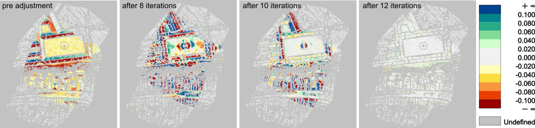
Figure 8: Mosaic of strip differences a priori (left), after 8 and 10 iterations, and a posteriori (right).

Example 2: Hybrid laser/image orientation with loose images

This example calls Module StripAdjust to execute a rigorous adjustment of 2 pairs of cross-wise overlapping flight strips (i.e. subsets of 4 strips in total) plus six aerial images. The orientation of images in object space is independent of strips and trajectories, and the given image timestamps are ignored. Note that the provided images are downsampled overviews and cannot be used in combination with the given interior orientation (e.g. for image matching).

opalsStripAdjust -utm.zone 33 -.hemisphere north -adjustment.voxelSize 5 -.maxIter 20 -strips.all.iFormat sdc -.oFormat odm -.scannerOrientation DFR -.trajectory.correctionModel bias -strips[0].inFile melk11.sdc -strips[1].inFile melk12.sdc -.trajectory.dX.sigma 0 -..dY.sigma 0 -..dZ.sigma 0 -..dRoll.sigma 0 -..dPitch.sigma 0 -..dYaw.sigma 0 -strips[2].inFile melk21.sdc -strips[3].inFile melk22.sdc -strips.normals.searchRadius 1.5 -images.all.extOri.X0.sigma 0.2 -..Y0.sigma 0.2 -..Z0.sigma 0.2 -images.all.oriFile melkImageTimestampsAndOrientations.txt -images[0].inFile melk122326.jpg -.obsFile melk122326_obs.txt -images[1].inFile melk122328.jpg -.obsFile melk122328_obs.txt -images[2].inFile melk122329.jpg -.obsFile melk122329_obs.txt -images[3].inFile melk124447.jpg -.obsFile melk124447_obs.txt -images[4].inFile melk124449.jpg -.obsFile melk124449_obs.txt -images[5].inFile melk124450.jpg -.obsFile melk124450_obs.txt -sessions[0].trajectory.inFile TrjMelk_utm33.txt -.iFormat trajectory.xml -.timeLag 0.0004 -cameras[0].intOri.c.value 9940.71 -..X0.value 5121.91 -..Y0.value -3842.75 -...distortion.rho0 4306 -correspondences.strip2strip.overlap 1 -.selection.samplingDist 5 -..rejection.maxDist 1 -...image2strip.dpSigPriori 0.5 

As in example 1, a configuration file or a python script can be used alternatively. The respective files are $OPALS_ROOT/demo/melkStripAdjust_Hybrid.cfg and $OPALS_ROOT/demo/melkStripAdjust_Hybrid.py. Given that the parent directory is the current working directory, these can be executed analogous to example 1:

opalsStripAdjust -cfgFile melkStripAdjust_Hybrid.cfg

And in Python:

python melkStripAdjust_Hybrid.py

Example 3: Hybrid laser/image orientation with coupled images

While the data used in this example is the same as above, we tie the images to the flight trajectory here. Apart from assigning each image to a strip, the only additional input needed with respect to the previous example are image time stamps. The initial forward intersection of image points into object space requires relatively good estimates of the camera mounting calibration parameters (lever arm and misalignment angles). Since they are not set here and exterior image orientations are provided, they are automatically estimated by Module StripAdjust.

Due to the small size of the data set, the image-specific exterior orientation correction parameters i.e. residual image shifts and rotations optimizing the image bundle block on top of direct georeferencing (trajectory and camera mounting), must be set constant to achieve meaningful scanner and camera mounting calibrations and trajectory corrections.

The following command reuses the cfg-file for the hybrid adjustment with loose images and adds the few additional parameters on the command-line:

opalsStripAdjust -cfg melkStripAdjust_Hybrid.cfg -maxIter 12 -images[0].strip 0 -[1].strip 0 -[2].strip 0 -[3].strip 2 -[4].strip 2 -[5].strip 2 -images.all.dExtOri.dX0.sigma 0 -..dY0.sigma 0 -..dZ0.sigma 0 -..dOmega.sigma 0 -..dPhi.sigma 0 -..dKappa.sigma 0

The following figure shows the improved relative strip differences compared to the laser-only case (cf. figure 8, right).

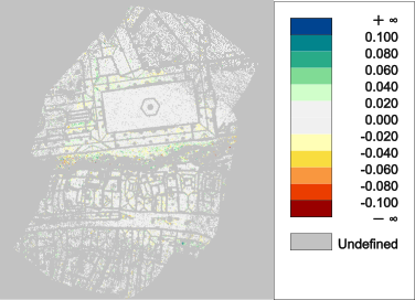
Figure 9: Masked strip differences after hybrid adjustment with coupled images.

References

Glira, P., Pfeifer, N., Briese, C., Ressl, C., 2015: Rigorous strip adjustment of airborne laserscanning data based on the ICP algorithm. In: ISPRS Annals of the Photogrammetry, Remote Sensing and Spatial Information Sciences, Volume II-3/W5, 73-80.

Glira, P., Pfeifer, N., Mandlburger, G., 2016: Rigorous Strip adjustment of UAV-based laserscanning data including time-dependent correction of trajectory errors. Photogrammetric Engineering & Remote Sensing 82 (12), 945-954.

Glira, P., Pfeifer, N., Mandlburger, G., 2019: Hybrid orientation of airborne lidar point clouds and aerial images. In: ISPRS Annals of the Photogrammetry, Remote Sensing and Spatial Information Sciences, Geospatial Week 2019, Enschede, NL (in press).

Author

pg, wk, mwimmer, gm

Date

24.03.2017