Technische Universität Wien
Orientation and Processing of Airborne Laser Scanning data
Department of Geodesy and Geoinformation - Research Groups Photogrammetry and Remote Sensing
The LiDAR measurement technology is well suitable for capturing electricity infrastructure. In particular power lines and power poles are often measured using airborne LiDAR platforms mounted on helicopters or planes. In case of smaller areas of interest also drones can be utilized. As shown in this use case below, OPALS can be used to classify cable points in a straightforward manner that were captured from a plane mounted LiDAR system. Those cable points are further segmented into individual parts between poles (this information allows estimating the sag of the cables, which is an important quality measure of the cable). Moreover, insulator and pole points can be segmented providing the geometric location of those objects.
Electricity provider need to secure the integrity of their infrastructure which also includes monitoring and cutting down vegetation close to power lines. Once a power line corridor has been fully classified, OPALS can also be used to estimate the distance between cable points and closest (vegetation) points.
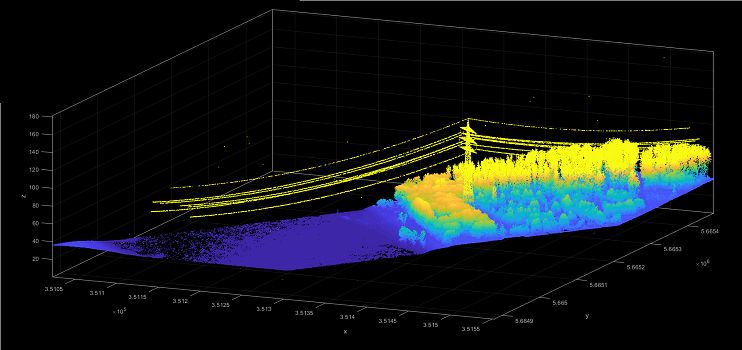
The ALS data which is used for the present use case includes power lines and its tower, water area, forest area, single trees and vegetation.
The use case data niederrhein.laz are located in the $OPALS_ROOT/demo/classify directory of the OPALS distribution and were captured by a Riegl LMS-Q560 Airborne Laser Scanner.
In the current data set, power lines can be extracted within 4 steps. After segmentation of power lines, bounding box of the tower can be extracted.
As a prerequisite the data needs to be imported into an ODM using the Module Import. Therefore, change into the $OPALS_ROOT/demo/ directory and run the following command:
Now, the powerline.odm file should exist in the current directory ($OPALS_ROOT/demo/). Due to the use of a region filter, only points in the powerline corridor are imported. Next, Module Normals is used to estimate a normal vector for each point.
When setting the storeMetaInfo parameter to maximum, not only the estimated normal vector but also to the eigenvalues and eigenvectors of the local structure tensor are stored by Module Normals. Needless to say, the number of neighbours and the search radius parameter will effect the neighbourhood definition and therefore, have significant influence of the estimation results. Especially, the search radius needs to be adapted for other sensors or data sets.
The eigenvalues from the normal estimation process can now be used, to compute a local linearity measure. Since Module Normals always sorts the eigenvalues (and eigenvectors) in descending manner, following formulation is utilized to estimate a linearity value between 0 (low linearity) and 1 (high linearity): \(\sqrt{1 - NormalEigenValue2 / NormalEigenValue1}\) (in literature also slightly different linearity definition can be found. see in the reference section for further details)
Using Module AddInfo, the linearity values are calculated and added to powerline.odm file as attributes. The greater the linearity value, the higher possibility to being a part of a power line.
Linearity value can show if a point is on a line. However, high linearity values not only represent power lines but also other linear objects such as trees in the data. Module Segmentation is used to find points which has very high linearity and small angle between the first eigenvector (=direction of largest extend of neighbouring points) in the local neighbourhood.
Module Module AddInfo is used to store segmented power line points as attribute _cableId.
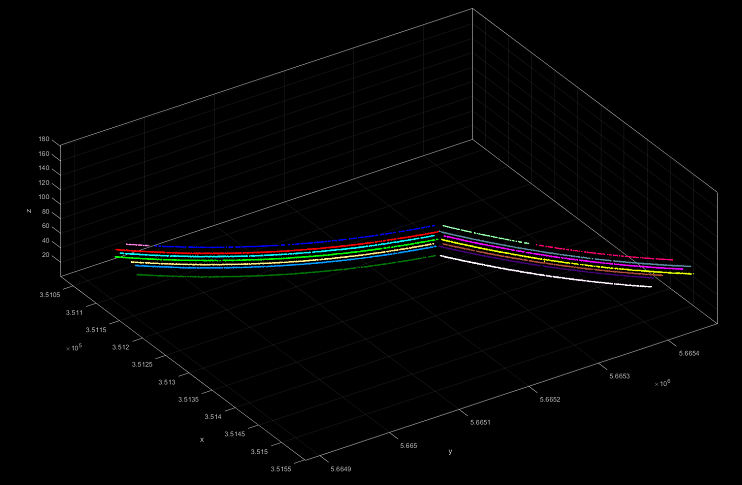
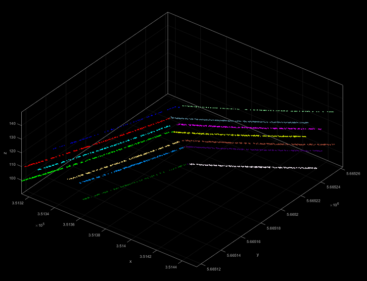
Most of the power line points could be segmented except the points which closed to tower. There are also some other missing sparse point groups between segments.
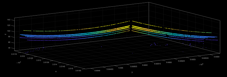
In the first segmentation, some power line points cannot be found but reliable power line points are detected as seen in Fig. 4. While normal estimation is performing, according to number of neighbours and search radius, normal vectors and eigen normal vectors are affected by position of neighbour points. Furthermore, linearity is also affected by these facts. Therefore linearity is getting reduced araund tower where normal vector direction changed dramatically. Considering the fact that reducing linearity, most of the lost powerline points are expected to located araund tower. To detect lost power line points, Module PointStats is used. On the other hand, in some cases power line points does not have high linearity value.
The following commands can be used iteratively. Fig. 5 shows points with _cableId after iterations.
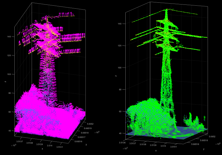
Missing power line points of first segmentation which are placed around tower can be used to detect tower. To find starting points around tower, Module PointStats is used. Neighbours that has no _cableId value of points which has a _cableId value are searched within a search radius.
For extraction of tower points, region growing based segmentation method is applied using Module Segmentation. Using starting points over tower, filtering points with _cableId and searching for points in a small 3d region with small normal eigen vector angle threshold allows to find tower points.
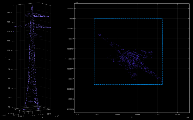
As clearly seen in Fig. 6, applied method is not able to find all tower points. Nevertheless, most of points of tower can correctly be detected. So extracted tower points are convenient to find bounding box of the tower.
Melzer, T., Briese, C., 2004: Extraction and modeling of power lines from als point clouds. In Proceedings of 28th Workshop of the Austrian Association for Pattern Recognition (ÖAGM), pp. 47-54.
Chehata, N., Guo, L., Mallet, C., 2011: AIRBORNE LIDAR FEATURE SELECTION FOR URBAN CLASSIFICATION USINGRANDOM FORESTS, IAPRS, Vol.XXXVIII, Part 3/W8, pp. 207-212
Weinmann, M., Jutzi, B., Hinz, S., Mallet, C., 2015: Semantic point cloud interpretation based on optimal neighborhoods, relevant features and efficient classifiers, ISPRS Journal of Photogrammetry and Remote Sensing, 105, ISSN 0924-2716, pp. 286-304
 1.8.17