Technische Universität Wien
Orientation and Processing of Airborne Laser Scanning data
Department of Geodesy and Geoinformation - Research Groups Photogrammetry and Remote Sensing
Mount Rainier is frequently affected by various types of natural hazards. Those hazards range from lava flows, landslides, rockfalls, earthquakes, pyroclastic flows to lahars. The latter pose the greatest hazard from Mount Rainier. Lahars, also known as volcanic mudflows or debris flows, are large flows of eruption or hydrothermal origin that benefit from abundant ice, loose volcanic rock and surface water at Mount Rainier. Lahars at Mount Rainier vary in their fluid content but can travel as fast as 70-80 km per hour and may flow up to 100 km downstream to Puget Sound. At least 60 lahars have flowed off Mount Rainier into its draining river valleys in the past 10,000 years, with the largest events occurring about every 500 years (Pinsker, 2004). In response to the lahar-hazard, warning systems have been implemented. Before even thinking about such installations, the areas most susceptible to specific hazardous events have to be identified. Physically based modelling approaches are capable of predicting lahar runout. Such models have in common that they need proper and high quality topographic data. High resolution LiDAR produces raw data perfectly suitable for such analyses. In the following chapters some guidance is given for a typical workflow in geomorphological research to produce some ready-to-use topographic raster data with OPALS.
LiDAR techniques have been extensively used for topographic surveys since the mid-1990s. Data acquisition was first performed by means of ALS (airborne laser scanning), whereas TLS (terrestrial laser scanning) emerged as a valuable field in earth sciences since approx. 2000 (Jaboyedoff et al. 2012). Existing geomorphological applications encompass landslide and rockfall dynamics (Teza et al., 2008; Abellán et al., 2009, 2010), coastal cliff erosion (e.g. Rosser et al., 2005), braided rivers evolution (e.g. Milan et al., 2007), river bank erosion (e.g. ONeal and Pizzuto, 2011) or debris flows impacts (Schürch et al., 2011). Höfle & Rutzinger (2011) published an extensive article about the applications of airborne LiDAR in geomorphological applications.
Data acquisition by LiDAR techniques comes with the benefit of generating full 3D land surfaces. However, when it comes to analyses of multi-temporal datasets, the most common method of point cloud comparison in earth sciences is still the Digital Elevation Model (DEM) of difference (DoD) technique (Lague et al., 2013). That means that two registered point clouds are gridded to generate DEMs which are then differentiated on a pixel-by-pixel basis. Thus, the vertical distance between two corresponding raster cells is taken into account as a measure of surface change. Although a very fast technique that comes with a simple and well known data structure, it has the huge drawback of being only a 2.5D representation of the land surface, thus decreasing information density proportionally to surface steepness (i.e. vertical surfaces such as cliffs or rock faces) cannot be accounted for in a grid representation. Contrary, full 3D analyses are limited to direct point cloud processing techniques (such as C2C, C2M or M3C2) that do not depend on gridding or meshing the original data (Lague et al., 2013). Yet, applications that directly make use of the 3D point cloud are not as abundant, which can be explained by the lack of suitable software tools providing management and analysis functionality as well as direct integration with standard GIS and remote sensing software (Höfle & Rutzinger, 2011). Nonetheless, rasterized point cloud derivatives are appropriate by all means with respect to the research question raised, hence the dominance of raster-based applications.
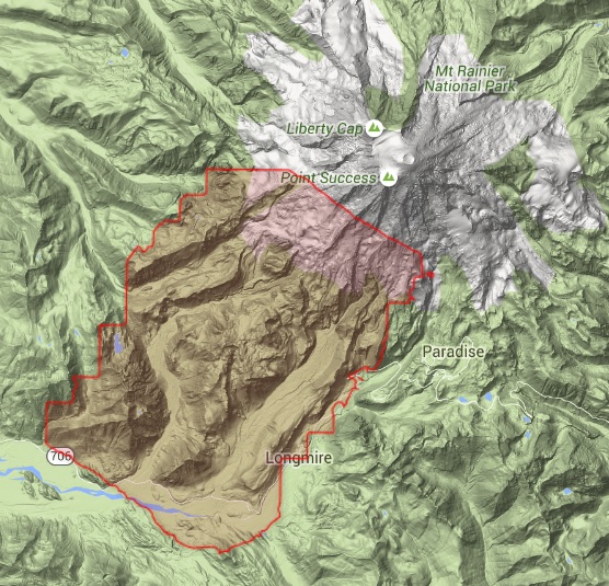
In this use case we try to exploit the potential of OPALS as a tool for explorative data analysis and the preparation of raster data for subsequent model applications. Pfeifer et al. (2013) give some in-depth insight into the OPALS framework. For any question that arises while working with OPALS, an extensive use of the OPALS module descriptions that are available online is highly recommended. The data used here is obtained from OpenTopography, a high-resolution topography data repository that offers point cloud data under a free license (public domain). The raw data of the southwest flank of Mount Rainier can be directly downloaded from here. Fig. 1 shows the area covered by the point cloud. As for the point cloud download, the LAS file format was chosen (download in a generic ASCII file format available too). The survey that took place from August 28, 2012 to September 1, 2012, covers an area of 123 km². Processing the entire point cloud would be quite time demanding, thus, we only use a subset of the point cloud for fast and easy processing. You can download the subset used for this use case (UseCase_geomorph_MtRainer.7z) from the OPALS download page.
In a first step, we derive different topographic models from our 3D point cloud. The most frequently used model for geomorphological applications is the Digital Terrain Model (DTM) representing the elevation of the ground surface. In contrast to the DTM, a Digital Surface Model (DSM) represents the elevation of the topmost surface (e.g. treetops, roofs). A DSM can be derived by the determination of the highest point within a defined raster cell (DSMmax) or the determination of the DSM heights based on moving least squares interpolation, e.g. moving planes (DSMmls). In order to obtain a simple DTM, we will use the lowest point within a raster. Depending on the research question, more sophisticated vegetation removal tools might be required. Lastly, a simple method is applied to fill data gaps in the DTM. This is necessary for every physical based or numerical model applied later on that makes use of the DTM as the topographic base, especially when any kind of flow propagation (overland flow, river discharge, debris flow propagation, etc.) is involved.
The OPALS modules involved here are as follows:
For generating a new ODM:
Generating a digital elevation model works with both, opalsCell and opalsGrid. The aim of Module Cell is to derive raster models by accumulating specific features (min, max, mean, etc.) of a selected input data attribute (z, amplitude, echo width, etc.), while opalsGrid derives digital elevation models in regular grid structure using interpolation techniques. The aim of Module Grid is to derive digital surface models (DSM/DTM) in regular grid structure using simple interpolation techniques like nearest neighbour or moving planes. This means that opalsCell derives only a single raster pixel value based on all valid values for a selected attribute within a raster cell (in our case the z-coordinate that represents the height), whereas opalsGrid interpolates over all values within a user-defined local neighbourhood. Consequently, the height estimation based on opalsCell may be more accurate in rough areas (e.g. canopy), but less robust with respect to errors resulting from outliers.
For derivation of GIS raster data we can now use:
Mind that you can specify different features (max, min) in one line. In case no attribute is specified, OPALS uses the default attribute z. The output files are named accordingly (dsm_3m_z_max.tif and dsm_3m_z_min.tif). For the DSM generation with opalsGrid we used a moving (tilted) plane interpolation, yet there are more interpolation methods available in OPALS.
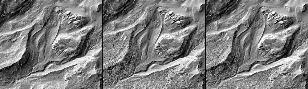
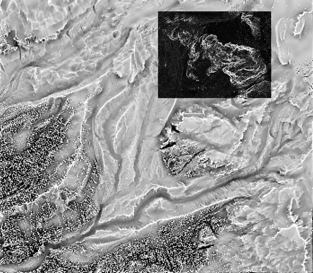
For a better visualization of the digital elevation models, we use opalsShade (cf. Fig. 2). Hill shading is a method to visualize a surface grid model by illumination using an artificial light source shining from a certain direction. However, all subsequent analyses are based on the DSM/DTM only.
Shading a DSM/DTM is straight forward, yet there are some more options available in OPALS if required (with respect to the shading method or the artificial sun position).:
When working with physical based slope stability models, it is often advisable to separate forested from non-forested areas to account for the stabilizing effects of trees (intercepted precipitation, root cohesion, etc.). Thus, it would be interesting to extract all trees from the study area. Our data only contains x,y and z coordinates and no other attributes that give any information on a potential vegetation cover (e.g. echo with from full-waveform LiDAR data). Therefore we have to make an assumption, namely that we consider forested areas only as such with relative heights greater than 3 m with respect to the lowest point in the corresponding raster cell.
This requires two steps:
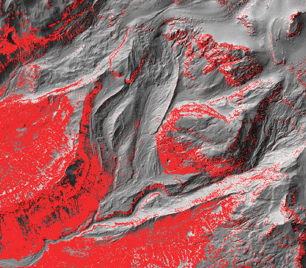
In step 1 we produce a normalized DSM (nDSM) by subtracting the DTM from the DSM. The aim of Module Algebra is to derive a new grid dataset by combining multiple input grid datasets. The new grid values are calculated by applying an algebraic formula using the grid values of the respective input grids. The formula is passed as a string in generic filter syntax. Apart from these basic operations, conditional statements are of crucial importance for the construction of complex formulas. For example in step 2 we want to generate a raster that only contains the data from step 1, if the relative height of a raster cell is higher than 3 m, otherwise the raster cell is set to no data. Please note that r[0] represents the first input raster, r[1] the second one. Fig. 3 shows the result in red (superimposed to the DTM in a GIS).
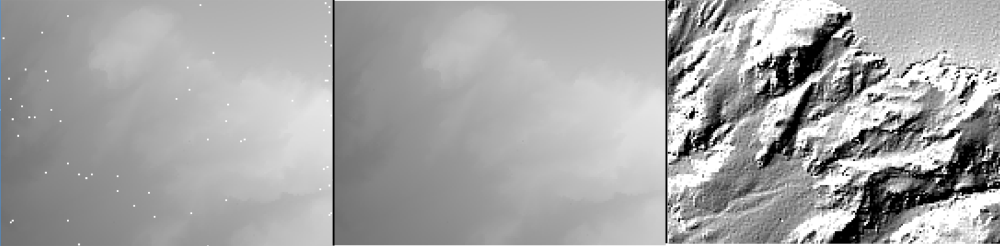
When processing point cloud data into a regular raster, gaps may occur due to occlusions in the original point cloud (mainly an issue with terrestrial laser scanners) or due to variations in point density that affect the interpolation (e.g. grid size smaller than point spacing). However, for many geomorphological applications, especially when applying distributed models that rely on a raster input for the base topography, the DTM should be gap-free.
OPALS provides a possibility to remove gaps by smoothing the raster data. This is done by averaging the height in a certain local neighbourhood (kernel). Therefore, we use the opalsStatFilter module. The aim of Module StatFilter is to perform statistical filtering of raster datasets with respect to a user-defined kernel area. However, filtering an entire raster surface would lead to alterations that are undesirable for all non-empty raster cells. Consequently, we want to fill the gaps in the DTM by taking the information from the smoothed DTM while not changing all other cell values at all. This requires three successive steps:
Although digital elevation models are the most commonly used LiDAR product, morphometric derivatives (such as slope, aspect, surface roughness) greatly improve the topographic interpretation for natural hazard management. Here some simple steps are shown how to produce such morphometric parameters.
Slope and aspect (the compass direction that a slope faces) are to commonly used parameters in geomorphological analyses. Slope is usually the most significant and sensitive parameter in physically based modelling, while aspect can be an evenly important parameter, depending on the research question (e.g. when micro-climatic influences are of importance). The opalsGrid module offers integrated features that easily generate such raster maps (Fig. 5). Those features are slope and expos.
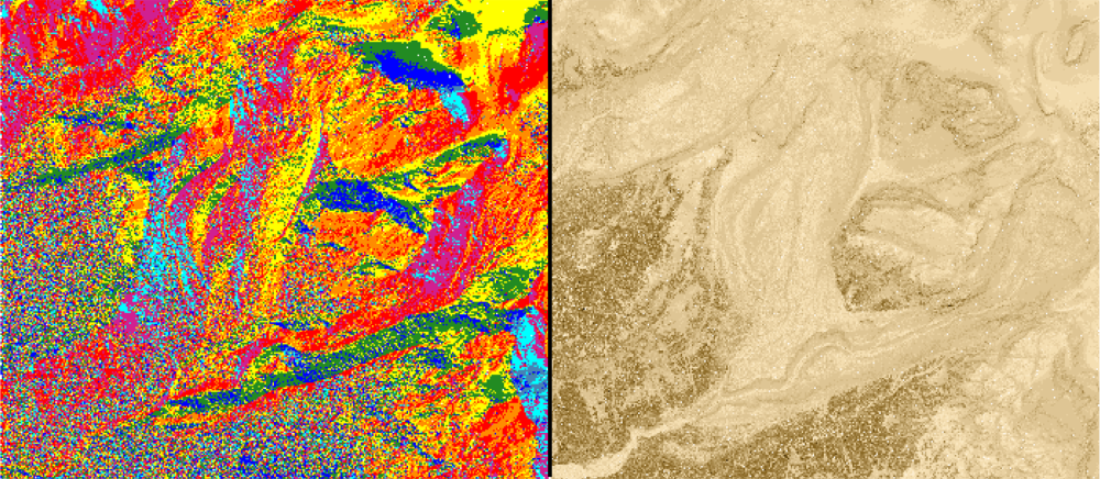
Surface roughness is an important geomorphological parameter as it heavily influences any flow processes (such as lahars, debris flows or river floods). In OPALS, the roughness (sigmaZ) is expressed as the standard deviation of the interpolated grid height (with movingAverage or movingPlanes interpolator only). Same as with the slope and aspect, it is contained as a feature in the opalsGrid module. Another measure of convexity/concavity is contained in the module opalsOpenness (Fig. 6).
 1.8.17