Technische Universität Wien
Orientation and Processing of Airborne Laser Scanning data
Department of Geodesy and Geoinformation - Research Groups Photogrammetry and Remote Sensing
Estimate the Diameter at Breast Height (DBH) based on 3D point cloud data (ODM).
In forestry the diameter at breast height is an important measure for various estimation models and applications. Although, the model was primarily designed for stem estimation it can also be applied for modelling artificial objects like pipes or other cylindrical and conical objects. Based on given approximations (3D point, axis and radius) the module applies robust least-square fitting of cylinders or cones to neighboring points of the approximate 3d point. Hence, for each stem a separate entry within the approximation file is required. Beside the standard single fit mode, the module can also trace the stem in and opposite to the axis direction respectively (parameter trace). In trace mode the parameters patchLength, overlap and the results of the previous fit are used to compute new approximations for the next fitting step. The actual output is a shape file with 3d circles at representative position with additional statistical information of each fit. Furthermore, from python and C++ all results can be directly accessed as a vector of stem objects by requiring the output parameter outResults (see here for further details).
The provided approximations are not only used as initial values for the linearized least-square models but also for sub-selecting relevant points for the actual fit. As shown in Figure 1, Module DBH uses an extended cylinder for the data selection, where \( P_1 \) (first point of the stem approximation) is a the center of the selection cylinder, the cylinder axis \( \vec{a} \) is aligned with \( P_1 \) and \( P_2 \) (second point of the stem approximation) and the cylinder height is equal to patchLength. Whereas vertical axis approximations are appropriate for trees in general, in rare cases of titled or horizontal (e.g. dead wood) stems with many outlier points in the surrounding (e.g. undergrowth, shrubs or nearby trees) it might be necessary to have more accurate non-vertical axis approximations since this will select more relevant stem points.
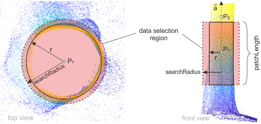
The radius of the data selection cylinder can be controlled by the searchRadius parameter. The definition of an appropriate formula is essential to get correct least-square fits, since too small values may excluded correct stem points from the fit. On the other hand, oversized searchRadius values may introduce too many false points precluding the implemented outlier detection to work (correctly). So depending on the input data and the accuracy of the approximations, it can be necessary to adapt the searchRadius formula. Module DBH provides the approximate point (x, y and z) radius (_r) and axis (_axisX, _axisY and _axisZ), the stem and trace id (_StemId and _TraceId) to the formula allow defining fine adoptions to the searchRadius values. In case the formula returns invalid (see Generic filter for further details), no data selection and consequently, no fit will be performed (in trace mode the iteration in the current direction is stopped).
As mentioned before, ModuleDBH is capable of tracing stems in and opposite to the axis direction. This feature can be used to either extract a more detailed representation of the corresponding tree or to get the stem diameter at different height(s) than the initial approximation point height. Especially in case of dense undergrowth extracting initial stem position higher than breast height can help to increase robustness. Then, using down tracing the stems allows extracting the diameter at the sought-after height. To enable trace mode in axis direction set the first value trace to true. The second value controls the opposite axis direction tracing. Hence, it is possible to activate the two tracing directions independently. In case the axis direction is always oriented upwards (P2 is always above P1 as in the approx file below) the first trace flag matches the growing direction of the trees.
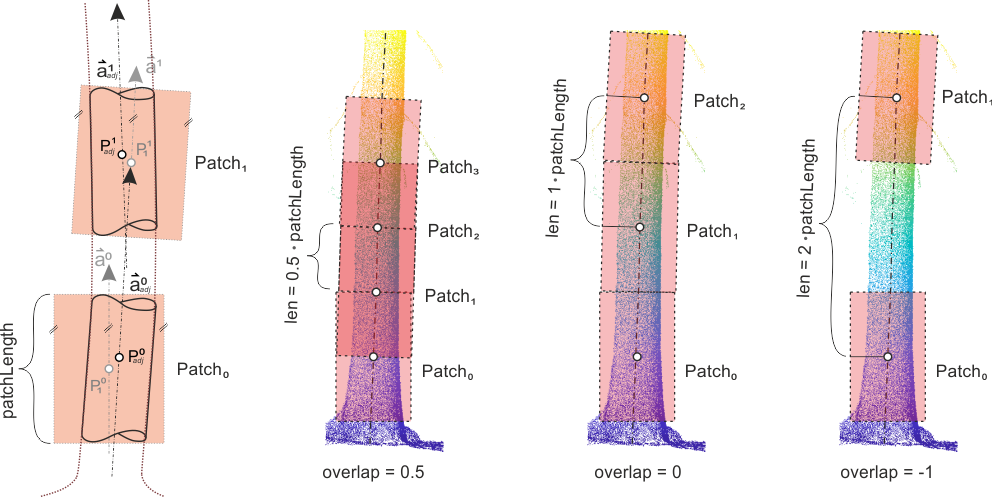
As shown on the left in Figure 2 the adjusted results of the previous patch are used as approximations for the next patch. The spacing between consecutive patches are controlled by the overlap parameter but also depends on the patchLength. An overlap of 0.5 results in 50% overlapping patches, whereas an overlap of 0 leads to touching patches. The length of the shift vector between consecutive patches is computed by
\( len = (1-overlap) \cdot patchLength \)
The module stops tracing in one direction if two consecutive fits are classified as incorrect. Either the least-square adjustment itself did fail (e.g. no convergence was achieved, not enough input data were selected, etc.) or the continuity check discard the results. This continuity check use several heuristics to decide whether the current results fits to the previous result. The result is discard if,
Details on which criteria stop the iterations will be logged, if the file or screen log level is set to debug (see Logging / Error Handling for further details).
User can either prepare the approx file in the default ASCII format or a corresponding OPALS format definition file can be specified. In the default format two points and the approximate radius must be defined for each stem
where the first point ( \( pt1 \)) is used as center of the selection region and the approximate axis points from the first to the second point ( \( a = pt2 - pt1 \)). Since lines with a leading '#' character are ignored, it is possible to place comment or header lines within the file but also, deactivating single stem approximations by inserting an '#' character at the beginning of the corresponding line.
The usage OPALS format definition adds some extra feature that maybe valuable in certain situations:
The columns of an approximation files that are interpreted in the following way:
| Attribute | Interpretation | Remark |
|---|---|---|
| x,y,z (=default coordinates) | first point | |
| _x1, _y1, _z1 | first point | alternative coordinate definition |
| _x2, _y2, _z2 | second point | |
| _axisX, _axisY, _axisZ | axis vector | alternative to second point |
| _r | radius | |
| _radius | radius | alternative to attribute _r |
| _filter | individual filter | optional data filter for each stem |
| [...] | pass through columns | optional |
For ModuleDHB a valid OPALS format definition files must contain an approximate radius value and
for each stem entry. Individual filters and pass through columns are optional. Although the approximation will be stored in an ASCII file in general (due to the low number of stem approximation the poor IO performance of ASCII files is irrelevant), the OPALS format definition concept is flexible enough to support binary or even LAS/LAZ as long as the necessary data columns are provided. How to use pass through columns and Individual filters is shown in exampe 2.
For the cylinder and cone fit the module uses the functional models described by Lukács et. al. (1997). Using robust least-squares strategies the method can cope with gross errors and therefore classifies points into in- and outliers. To avoid extrapolation, the final resulting point ( \( P_{adj} \)) is computed by orthogonal projection of the center of gravity (CoG) of all inliers onto the adjusted axis. In other words, intersecting the adjusted cylinder/cone axis with plane e (is orthogonal to the axis and contains the inlier CoG) gives the representative point \( P_{adj} \).
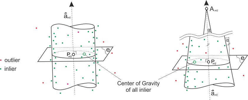
The results of all successful fits are written to a shape and ASCII file (see parameter outFile). The content of both files is basically the same with one exception. As geometry object the shape file uses a visual representation of the fitted model, namely the 3d circles as shown in Figure 3, rather than just a point representation of \( P_{adj} \). Nevertheless, the coordinates of \( P_{adj} \) are attached as attributes to the circle object. When fitting a cone also the convergence angle (=half of opening angle of cone) is output. In case the cone radius is decreasing in axis direction (i.e. the cone apex is above plane e based on the axis direction, as in Figure 3), the value is positive. If the radius is increasing when advance in axis direction, the convergence angle will be set negative.
| Attribute | Interpretation | Remark |
|---|---|---|
| Id | output id | unique identifier needed to fulfill the shape file specification |
| StemId | input stem id | matches the approx input stem id |
| TraceId | trace id | 0 for the initial fit, increasing while forward tracing and decreasing (i.e. negative numbers) while backward tracing |
| x, y, z | coordinates of \( P_{adj} \) | |
| r | adjusted radius | |
| ax, ay, az | adjusted axis vector | |
| convAngle | convergence angle | set for cone fits only: it is the angle between the cone generatrix and the cone axis. The value is set positive if the cone radius is decreasing when advancing in axis direction and negative if it is increasing. This columns allow differentiating between cylinder and cone fits. |
| offsetX, offsetY, offsetZ | offset vector from the approximate point to the adjusted axis | |
| dr | correction of approximate radius value | |
| RadialDev | radial deviation based on inlier points | |
| Redundancy | redundancy of adjustment | |
| nObs | number of adjustment observations (i.e. points) | |
| nUsed | number of used inlier observations (i.e active points) | |
| [...] | pass through columns | optional |
Beside the output files it is possible to directly access the result from Python and C++ by querying the output parameter outResults. The returned object is a vector of opals::StemModel objects. Each stem object in turn stores at least one successful model fit (or multiple fits in trace mode). Each successful fit is represented as opals::StemEntry. Therefore, it is possible to further process or analyse the full results without parsing any result file.
The data used in the following example are located in the $OPALS_ROOT/demo/dbh directory. This simple example shows a how the module can be used based on given stem approximation.
As a prerequisite, the TLS point cloud of four trees must be imported into the ODM. To achieve that, change to the demo/dbh directory and type:
Now, run the following command
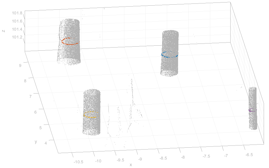
which outputs the shape file trees_results.shp and trees_results.txt. The ASCII file contains the same results but in human readable form. Using opalsView a quick visual 3D check of the results can be performed by runing
and adding the shape file to the view:
The module allows passing through columns from the approximation to the result files. This feature is useful for preserving pre-computed information or properties of individual stems in the resulting products as shown below. Furthermore, the user can provide individual filter for each stem which is a high-end feature that is only rarely required. Nevertheless, its mode of operation is shown in this example. First, a segmentation of the stem points is performed by the following command,
which segments the 4 stems and 6 branchs within the specified height range. By sorting the segments by their point size, it is secured that the segment ids (attribute segmentId) result from 0 to 3. Assuming known tree heights (pass through attribute), approximation of the stem centers and their corresponding segement id, an approximation file for the four trees can be prepared:
The individual filters secure that only the corresponding segmented stem points will be used for stem fitting, which eliminats outliers and non-stem points for the actual adjustment step. To feed this information into the Module DBH, a corresponding OPALS Format Definition is required.
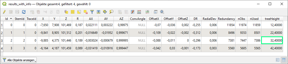
Columns that do not serve as stem approximations, as described above, will be passed through to the result output table (treeHeight in this case). The OFD-xml file needs to be set as aFormat parameter.
The command above will create results_with_info.shp which containes the following attribute table
The examples above are based on known/given stem approximations. But in general this information is not known in advance. In this extended example, a complete workflow starting from the raw 3D point cloud to the final DBH results including a method for extracting approximations is shown.
Assuming that the 3D point cloud has been imported into an ODM, one needs to first compute a DTM. This helps to subselect the relevant stem points but is also required to determine the breast height for each stem (typically 1.3m above ground). A simple method that results in approximated DTM is to selected the lowest point within 2D cells. The cell size must be selected that large that at least one ground point lies within each cell. Especially, in steep terrain the resulting model will be of low quality, but for the stem fitting it might be good enough.
To compute a high quality DTM one can use Module RobFilter or Module TerrainFilter (not included in the stable release yet) to classify ground points first, and then compute a detailed and accurate DTM, as shown be the following command sequence
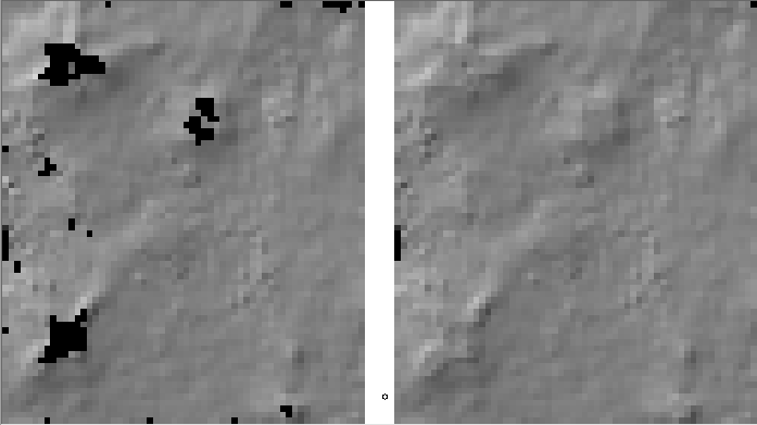
Using Module FillGaps unwanted holes can be filled to get a continuous model as shown in Figure 6.
Next, we computed the attribute normalizedZ for all points which helps to subselect relevant stem points and for finding robust DBH approximations.
In the following steps, we pre-filter stem point candidates and export them into a new ODM (trees_sub.odm) to increase robustness and processing speed. We consider echos that have a normalized height between 0.4 and 3m and which are last echos (in TLS solid bark echos are typically last echos). To further increase robustness also the vertical distribution of the points is considered using Module Cell. The vertical range and point count within 5cm 2D cells are computed and attached as attributes to the points. Echos are not consider (as stem points) if the vertical range and point count is less than 1m and 50, respectively.
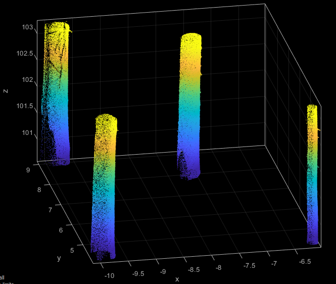
As shown in Figure 7 the previous filter step results in a good pre-selection of possible stem points.
Now its time to extract the actual stem approximation which can be done by using a small python script. The script utilises Module Segmentation to segment each stem using conditional clustering. The CoG of each segment and an estimated radius derived from the x- and y-extend of the segments are stored within a new approximation ODM. Although, the segment CoG can be shifted compared to stem center (especially if the stem has not been fully covered for all sides), this approximation error is usually uncritical for the subsequent process.
The height value, however, needs to be taken from the DTM rather from the segment itself. Since the DBH measure usually refers to the highest surface point in the stem vicinity, the height determination requires some additional processing. Therefore, the DTM is imported as additional point cloud into the approximation ODM. Then, the highest DTM point is determined within in a 0.25m radius to the stem approximation and attached as attribute _ZMax using Module PointStats. Finally, the actual DBH height is computed by adding 1.3m to _ZMax and stored in attribute _z1 by a corresponding Module AddInfo command. In this data set the stems are nearly vertical, which is why the second point of each stem approximation is simply set 1m above the base point (see attribute _z2). For death wood or titled stems better axis approximation might be necessary.
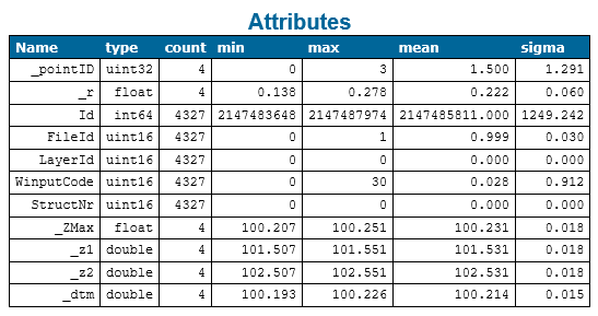
After the command sequence above the ODM contains all necessary information (see Figure 8) to write the actual approximation file.
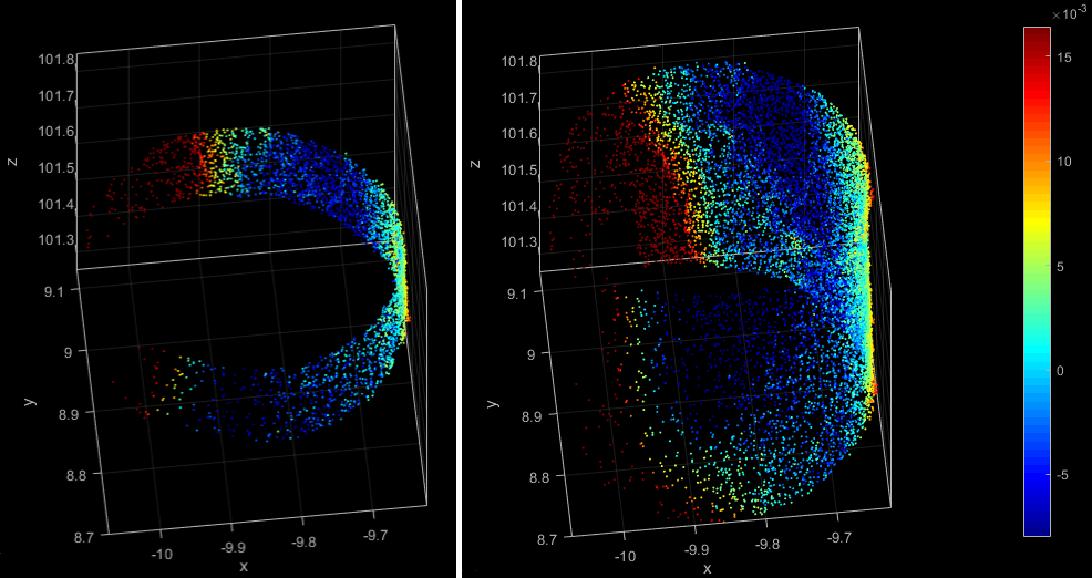
Once, the approximation file has been written, Module DBH can be called. When testing and evaluating different parameters and geometry models as shown below, it can be useful to additionally output fitting ODMs (see parameter byproduct). Those ODMs contain all points the where selected for fitting from the input ODM. Pointwise values computed during the robust least-squares adjustment are attached to each point, so e.g. detected outliers, the adjusted point sigma and the residual value can be easily visualised.
The signed fitting residuals of the first stem of the two module runs from above are visualised in Figure 9. Whereas the different patch length is easly visible, the effect of the different fitting model is hardly recognisable since the stem is narrowing very little over the seletect section.
GM: Idee für Abschlußsatz?
Bruggisser M., Hollaus M., Kükenbrink D., Pfeifer N., 2019, Comparison of forest structure metrics derived from uav lidar and als data, ISPRS Ann. Photogramm. Remote Sens. Spat. Inf. Sci., IV-2/W5, pp. 325-332, 10.5194/isprs-annals-IV-2-W5-325-2019
Bruggisser M, Hollaus M., Otepka J., Pfeifer N., 2020, Influence of ULS acquisition characteristics on tree stem parameter estimation, ISPRS Journal of Photogrammetry and Remote Sensing, Volume 168, pp. 28-40, ISSN 0924-2716, 10.1016/j.isprsjprs.2020.08.002
Lukács, G., Marshall, A. D., Martin, R. R., 1997, Geometric least-squares fitting of spheres,cylinders,cones and tori.
Wieser M., Hollaus M., Mandlburger G., Glira P., Pfeifer N., 2016, ULS LiDAR supported analyses of laser beam penetration from different ALS systems into vegetation, ISPRS Ann. Photogramm. Remote Sens. Spat. Inf. Sci., III-3, pp. 233-239, 10.5194/isprsannals-III-3-233-2016
 1.8.17